
Introduction
These two words — accuracy and precision — are used interchangeably in everyday conversation. Someone who hits a target consistently is called both accurate and precise without much distinction. In physics, this casual equivalence breaks down completely. Accuracy and precision measure two fundamentally different properties of a measurement, they fail in different ways, they require different remedies and confusing them leads to wrong conclusions about the quality of experimental data.
This article draws that distinction carefully. Not as a vocabulary exercise, but as a conceptual foundation — because understanding the difference between accuracy and precision is what allows a physicist to look at a set of measurements and correctly diagnose what went wrong, what can be fixed and how much the results can be trusted.
The Core Distinction
Here is the difference stated as directly as possible:
Accuracy is how close a measurement is to the true value of the quantity being measured.
Precision is how close repeated measurements are to each other — how reproducible the measurement is.
These are independent properties. A measurement can be:
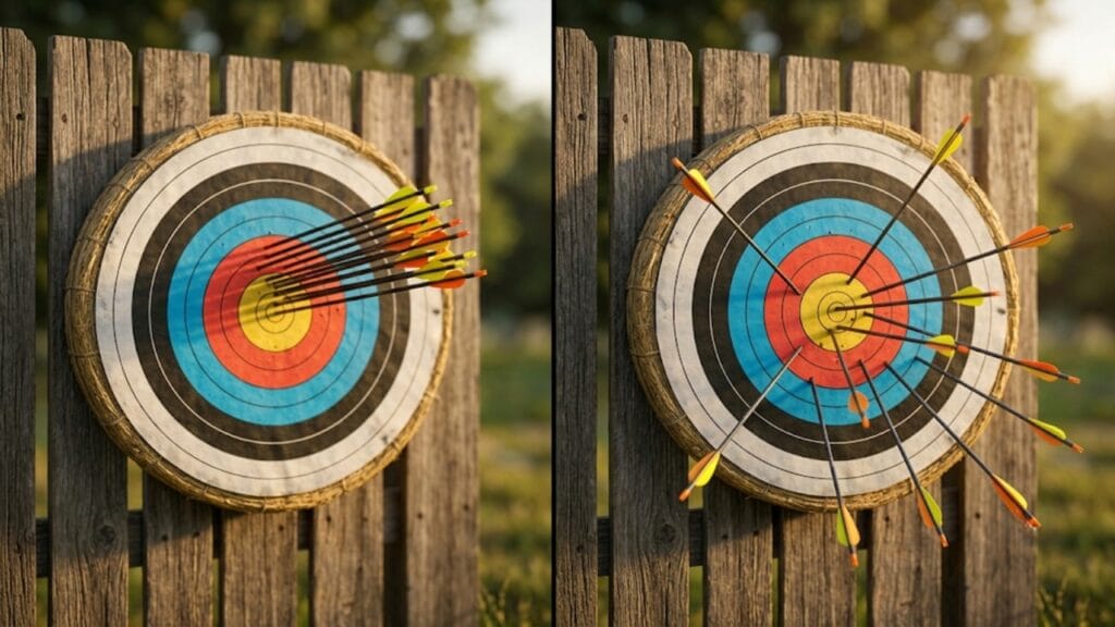
- Accurate and precise: All readings cluster tightly around the true value.
- Precise but not accurate: All readings cluster tightly, but around the wrong value.
- Accurate but not precise: Readings scatter widely, but average to the true value.
- Neither accurate nor precise: Readings scatter widely and do not average to the true value.
The fourth case — neither accurate nor precise — is straightforward experimental failure. The third case — accurate but not precise — describes an unbiased instrument with high random error. The second case — precise but not accurate — describes a biased instrument or method and is the most dangerous: it produces results that look reliable because they are reproducible, while concealing a systematic error that shifts all readings away from truth.
This is why precision without accuracy is, in some respects, worse than imprecision. A scattered set of readings signals a problem clearly. A tightly clustered set of wrong readings appears trustworthy.
Formal Definitions
Accuracy
Accuracy is a measure of how close the result of a measurement is to the true or accepted value of the quantity being measured.
Quantitatively, accuracy is often expressed through absolute error or percentage error:
\[ \text{Absolute Error} = |\text{Measured Value} – \text{True Value}| \]
\[ \text{Percentage Error} = \frac{|\text{Measured Value} – \text{True Value}|}{\text{True Value}} \times 100\% \]
A measurement with low absolute error and low percentage error is highly accurate. Accuracy is limited primarily by systematic errors — consistent biases that shift every reading in the same direction.
Precision
Precision is a measure of how reproducible repeated measurements are — how closely they cluster together, regardless of whether they cluster around the true value or not.
Quantitatively, precision is expressed through the spread of readings, most commonly through mean absolute error or standard deviation:
\[ \overline{\Delta x} = \frac{\sum_{i=1}^{n} |x_i – \bar{x}|}{n} \]
A measurement with small \( \overline{\Delta x} \) is highly precise — readings are tightly grouped. Precision is limited primarily by random errors and the least count of the instrument.
[Learn more about Absolute Error, Relative Error and Percentage Error: A Complete Guide]
The Four Cases: Visualized Through Measurement Data
Consider a physicist measuring the boiling point of pure water at standard atmospheric pressure. The true value is exactly 100.00°C. Four different scenarios illustrate the four cases:
Case 1: High Accuracy, High Precision
Readings: 99.97, 100.01, 99.99, 100.02, 100.00°C
Mean: 100.00°C. Spread: ±0.02°C.
The readings cluster tightly around the true value. This is the ideal outcome — a calibrated instrument operated with good technique in a controlled environment.
Case 2: High Precision, Low Accuracy
Readings: 98.42, 98.44, 98.41, 98.43, 98.42°C
Mean: 98.42°C. Spread: ±0.01°C.
The readings cluster extremely tightly — better precision than Case 1. But the mean is 1.58°C below the true value. Something systematic is wrong: perhaps the thermometer has a calibration error, perhaps the pressure is not at standard conditions, or perhaps the thermometer is not fully immersed. The tight clustering makes this easy to miss if you do not check against the true value.
Case 3: High Accuracy, Low Precision
Readings: 99.1, 100.8, 99.4, 100.6, 100.1°C
Mean: 100.0°C. Spread: ±0.7°C.
The mean is correct — the measurement is accurate in the sense that averaging produces the true value. But individual readings deviate by up to 0.8°C. Random errors dominate. This instrument or method has low precision. The result is useful only when enough readings are taken to average out the random scatter.
Case 4: Low Accuracy, Low Precision
Readings: 97.3, 101.8, 99.0, 102.4, 98.1°C
Mean: 99.7°C. Spread: ±1.8°C.
Wide scatter combined with a mean that does not quite hit the true value. Both systematic and random errors are significant. This measurement is of limited value without substantial improvement in technique and instrument calibration.
| Case | Accuracy | Precision | Error Type Dominant | Fix Required |
| 1 | High | High | Neither dominant | None — ideal outcome |
| 2 | Low | High | Systematic error | Calibration, method review |
| 3 | High | Low | Random error | More readings, better instrument |
| 4 | Low | Low | Both | Comprehensive improvement |

Error Types and Their Connection to Accuracy and Precision
The relationship between error types and the accuracy-precision distinction is direct and important.
Systematic Errors Affect Accuracy
Systematic errors shift all measurements consistently in one direction. They do not scatter readings — they bias them. A consistently biased measurement is reproducible (precise) but wrong (inaccurate).
Sources of systematic error:
- Instrument calibration error: A balance that reads 0.5 g too high on every measurement
- Zero error: A Vernier caliper with an undetected positive zero error
- Methodological bias: Consistently measuring a pendulum length to the top of the bob instead of its centre of mass
- Environmental factors: Temperature-dependent expansion of a steel ruler affecting every length measurement
Because systematic errors are consistent, taking more readings does not help. The bias persists in the average. The only remedies are calibration, zero error correction and methodological improvement.
Random Errors Affect Precision
Random errors cause individual readings to scatter unpredictably around the true value (or around the biased value, if systematic error is also present). They affect precision — how reproducible the measurement is.
Sources of random error:
- Observer estimation: Slightly different estimates when reading between scale graduations
- Environmental fluctuations: Air currents, temperature variation, vibration
- Timing variability: Reaction time differences in stopwatch measurements
- Instrument resolution: The finite least count of the instrument
Random errors can be reduced by taking more readings and averaging. The mean of \( n \) readings has a random uncertainty that scales approximately as \( 1/\sqrt{n} \). Doubling the number of readings reduces random uncertainty by a factor of \( \sqrt{2} \).
[Learn more about Top 5 Errors in Physics Measurements and How to Minimize Them]
Why Precision Without Accuracy Is Dangerous
This point deserves more than a passing mention. In experimental science, a set of precise but inaccurate measurements is the most common source of confidently wrong results.
Consider the historical measurement of the speed of light. Through the 19th century and into the early 20th century, physicists made increasingly precise measurements — readings that clustered more and more tightly around a central value — but that central value shifted systematically as experimental techniques improved. Each generation of measurements was more precise than the last, but systematic errors in earlier experiments had made those precise results consistently wrong.
The precision gave each set of measurements the appearance of reliability. The systematic errors — which varied from experiment to experiment — were not apparent within a single experimental campaign precisely because the readings were so consistent with each other.
This is why modern experimental physics reports both a random uncertainty (precision) and a systematic uncertainty (accuracy limitation) separately. A result quoted as:
\[ v_{\text{result}} = (299{,}792 \pm 3 \text{ (random)} \pm 10 \text{ (systematic)}) \text{ m/s} \]
carries more honest information than a result quoted with a single combined uncertainty — because it tells the reader which type of error dominates and what kind of improvement would most help.
Relationship to Significant Figures
Significant figures are the practical tool through which precision is communicated in a written measurement.
When you write a length as 4.53 cm, you are claiming precision to the nearest 0.01 cm — the last digit is significant and represents the estimated place. Writing 4.5 cm instead claims less precision: only ±0.1 cm.
Reporting 4.53000 cm when your instrument only resolves to 0.1 cm is a precision overclaim — you are asserting precision the measurement does not have. Reporting 4.5 cm when your instrument resolves to 0.01 cm is a precision underclaim — you are discarding real information.
Accuracy is a separate matter. A measurement reported as 4.53 ± 0.01 cm may be highly precise but systematically wrong if the true value is 4.70 cm. The significant figures communicate precision; the comparison with the true value reveals accuracy.
[Learn more about How to Find Significant Figures: Rules, Examples & Common Mistakes]
Real-World Examples
Example 1: GPS Navigation Systems
A GPS receiver reports your position as latitude 28.7041° N, longitude 77.1025° E. This position is precise to five decimal places of latitude and longitude — approximately ±1 metre of precision. But if the GPS satellites have systematic timing errors or the signal has been deflected by ionospheric refraction, the reported position may be consistently displaced by 5–10 metres from the true position.
The reading is precise (highly reproducible, well-specified) but not accurate (does not correspond to the true location). This is why differential GPS and other correction techniques exist — they eliminate systematic errors to restore accuracy without changing the instrument’s inherent precision.
Example 2: A Laboratory Balance with Calibration Drift
A digital balance in a chemistry laboratory reads consistently to ±0.001 g — three decimal places, excellent precision. Over time, the internal calibration weight shifts. Now the balance reads 0.15 g too high on every measurement.
Every reading is reproducible to ±0.001 g (high precision). But every reading is wrong by 0.15 g (low accuracy). A student using this balance to weigh a 10.000 g standard mass gets 10.150 g consistently. The consistency is not reassuring — it is evidence of the systematic error.
The solution is recalibration, not more readings.
Example 3: Measuring the Acceleration Due to Gravity
A student uses a simple pendulum to measure \( g \). They time 20 oscillations five times and get: 9.74, 9.78, 9.76, 9.75, 9.77 m/s². Mean = 9.76 m/s².
The readings are tightly clustered (precision: ±0.02 m/s²). But the accepted value of \( g \) at that location is 9.81 m/s². The 0.05 m/s² discrepancy suggests systematic error — possibly measuring the string length to the wrong point, using a non-spherical bob, or not accounting for air resistance. The high precision makes the systematic error more visible by contrast.
The student needs to identify and eliminate the systematic error, not take more readings.
Example 4: Blood Pressure Measurement
A blood pressure monitor reads 120/80 mmHg consistently across five measurements taken two minutes apart (high precision). The patient’s true blood pressure at that moment, measured by an invasive arterial line, is 135/90 mmHg.
The cuff measurement is precisely reproducible but systematically low — a common occurrence with automated cuff monitors in patients with arterial stiffness or peripheral vascular disease. The precision of the reading does not validate it.
This is why clinical guidelines recommend verifying monitor accuracy against a reference standard rather than simply relying on the consistency of multiple readings.
Example 5: Manufacturing Quality Control
A factory produces bolts with a specified diameter of 10.000 ± 0.010 mm. Two machines produce bolts measured by a precision calliper:
- Machine A: Diameters of 10.012, 10.011, 10.013, 10.012, 10.011 mm (mean 10.012 mm, spread ±0.001 mm)
- Machine B: Diameters of 9.998, 10.005, 9.993, 10.008, 10.001 mm (mean 10.001 mm, spread ±0.006 mm)
Machine A is more precise (tighter clustering) but less accurate — its mean is 0.012 mm above specification, which just barely exceeds the 0.010 mm tolerance. Every bolt from Machine A is slightly too large.
Machine B is less precise but more accurate — its mean is within specification, even though individual bolts vary more. Some bolts from Machine B may fall outside tolerance individually, but on average the machine is correctly centred.
This example illustrates why quality control engineers care about both accuracy (is the process centred on the target?) and precision (is the spread within the tolerance band?). The ideal — Machine C — would have both Machine A’s tight clustering and Machine B’s correct centring.

The Measurement Result: Combining Accuracy and Precision
In a well-conducted experiment, the final result carries information about both accuracy and precision. The conventional reporting format is:
\[ \text{Result} = \bar{x} \pm \overline{\Delta x} \]
Where \( \bar{x} \) is the mean (best estimate of the true value — relevant to accuracy) and \( \overline{\Delta x} \) is the mean absolute error (measure of spread — relevant to precision).
More sophisticated experimental reports separate the two components:
\[ \text{Result} = \bar{x} \pm u{\text{random}} \pm u{\text{systematic}} \]
The random uncertainty \( u{\text{random}} \) represents precision — it can be reduced by taking more measurements. The systematic uncertainty \( u {\text{systematic}} \) represents accuracy limitation — it can be reduced only by improving the experimental method, instrument calibration, or environmental control.
[Learn more about Measurement Uncertainty in Physics: What It Is and Why It Always Exists]
[Learn more about Propagation of Errors in Physics Calculations: Rules, Formulas & Examples]
How to Improve Accuracy and Precision Separately
Because accuracy and precision fail for different reasons, they require different remedies.
Improving Accuracy
- Calibrate the instrument against a certified reference standard before use
- Check and correct for zero error on all instruments with a zero point
- Review and standardize the experimental method to eliminate procedural biases
- Control environmental conditions — temperature, pressure, electromagnetic fields
- Use an independent measurement method — if two fundamentally different methods agree, systematic errors specific to each are unlikely to be common to both
- Compare with accepted values where available — a systematic discrepancy signals a systematic error to investigate
Improving Precision
- Take more readings and compute the mean — random uncertainty scales as \( 1/\sqrt{n} \)
- Use an instrument with a smaller least count — finer graduations reduce quantization uncertainty
- Eliminate environmental noise — vibration isolation, temperature stabilization, electrical shielding
- Improve observer technique — consistent eye positioning, consistent ratchet use, consistent timing method
- Use automated or electronic measurement — removes human reaction time and estimation variability
- Control the measurement conditions — ensure the quantity being measured is genuinely stable during the measurement period
[Learn more about How to Read a Measuring Instrument Correctly: Tips for Physics Lab]
Accuracy and Precision in the Context of Least Count
The least count of an instrument sets a hard lower bound on the precision of individual readings. No matter how carefully you read an instrument, you cannot extract information finer than its least count.
\[ \text{Minimum uncertainty per reading} = \pm \frac{1}{2} \times \text{Least Count} \]
or, by the more conservative school-level convention:
\[ \text{Minimum uncertainty per reading} = \pm \text{Least Count} \]
This is the instrument precision limit — the finest precision the instrument is capable of delivering. But it says nothing about accuracy. An instrument with a very small least count (high inherent precision capability) can still be systematically biased (low accuracy) if it is miscalibrated.
Conversely, a cruder instrument with a larger least count may be accurately calibrated — it delivers low precision but unbiased accuracy.
[Learn more about Least Count of Vernier Caliper and Screw Gauge: Formula & Calculation]
Common Misconceptions
Misconception 1: “More decimal places means more accuracy.”
Decimal places indicate precision of reporting — how finely the measurement is resolved. They say nothing about accuracy. A reading of 4.5328 m is more precise in its statement than 4.5 m, but if the true value is 5.0 m, neither is accurate. Accuracy requires agreement with the true value, not more digits.
Misconception 2: “A precise measurement is automatically reliable.”
Precision means reproducibility. A reproducible measurement with a systematic bias is reproducibly wrong. Reliability requires both precision (consistent results) and accuracy (results centred on the true value).
Misconception 3: “Taking more readings always improves the measurement.”
More readings improve precision by reducing the uncertainty in the mean. They do not improve accuracy. If a balance is calibrated 0.5 g too high, taking 100 readings instead of 5 gives you an average that is still 0.5 g too high — with better-determined precision around the wrong value.
Misconception 4: “Accuracy and precision are measured on the same scale.”
They are distinct properties that require different metrics. Accuracy is measured by comparison with the true value (absolute error, percentage error). Precision is measured by the spread of repeated readings (mean absolute error, standard deviation). They can be high or low independently of each other.
Accuracy vs Precision in Exam Questions
Both CBSE board exams and competitive papers (JEE, NEET) test this distinction in specific ways:
Type 1 — Definition question: “Distinguish between accuracy and precision with an example.” (2–3 marks, board)
Type 2 — Identification question: “A student measures the diameter of a wire as 1.22, 1.23, 1.22, 1.23, 1.22 mm. The true value is 1.46 mm. Comment on the accuracy and precision of the measurement.” The readings are precise (tight clustering) but inaccurate (mean 1.22 mm vs true 1.46 mm).
Type 3 — Error type linking question: “Which type of error affects accuracy and which affects precision?” Systematic errors affect accuracy; random errors affect precision.
Type 4 — Remedy question: “A student’s measurements are precise but inaccurate. What should they do?” Check and correct for zero error; recalibrate the instrument; review the experimental method. Do not take more readings — that will not fix a systematic error.
Summary: Key Differences at a Glance
| Property | Accuracy | Precision |
| Definition | Closeness to true value | Closeness of repeated readings to each other |
| Measured by | Absolute error, percentage error | Mean absolute error, standard deviation, spread |
| Affected by | Systematic errors | Random errors, least count |
| Can be improved by | Calibration, method correction, zero error fix | More readings, finer instrument, reduced noise |
| High value means | Results are close to the true value | Results are reproducible and consistent |
| Low value means | Results are biased away from the true value | Results vary significantly across repetitions |
| Can exist without the other? | Yes — accurate but scattered | Yes — precise but biased |
| More readings help? | No (for systematic error) | Yes (\( 1/\sqrt{n} \) improvement) |
Conclusion
Accuracy and precision describe two different things that can both go wrong in a measurement, for different reasons, with different remedies. Accuracy tells you whether you are hitting the right target. Precision tells you whether you are hitting the same spot repeatedly. Getting both right is the goal of every well-designed experiment.
The practical importance of understanding this distinction goes beyond exam answers. When experimental results disagree with theoretical predictions, the first diagnostic question is whether the discrepancy is systematic (an accuracy problem) or random (a precision problem). The answer determines whether the remedy is recalibration, more measurements, better technique, or a fundamentally different experimental approach.
Knowing the difference — precisely and accurately — is where good experimental physics begins.
Frequently Asked Questions
What is the difference between accuracy and precision in physics?
Accuracy is how close a measurement is to the true value. Precision is how close repeated measurements are to each other. A measurement can be precise without being accurate (consistent but wrong) and accurate without being precise (correct on average but scattered). High-quality experimental results require both.
Can a measurement be precise but not accurate?
Yes. This happens when systematic error is present. All readings cluster tightly together (high precision) but are consistently shifted away from the true value (low accuracy). A miscalibrated instrument is a classic example — it reproduces the same wrong reading reliably.
What type of error affects accuracy and what type affects precision?
Systematic errors — consistent, directional biases from instrument faults, zero error, or methodological problems — affect accuracy. Random errors — unpredictable fluctuations from observer estimation, environmental variability and instrument resolution limits — affect precision.
How do you improve accuracy in a physics experiment?
Improve accuracy by addressing systematic errors: calibrate the instrument, check and correct for zero error, standardize the experimental procedure, control environmental conditions and verify results against an independent measurement method. Taking more readings does not improve accuracy.
How do you improve precision in a physics experiment?
Improve precision by reducing random errors: take more readings and average them (precision improves as \( 1/\sqrt{n} \)), use an instrument with a smaller least count, eliminate environmental noise sources and improve observer technique to reduce estimation variability.
Why is high precision without high accuracy considered dangerous in science?
Because precise but inaccurate results appear reliable. Tight clustering of readings creates the impression of a well-controlled measurement, which can suppress the critical examination that would reveal the underlying systematic error. Scattered readings at least signal that something is wrong; precise but wrong readings may be accepted confidently and propagated into further calculations or published results.
What is the relationship between significant figures and precision?
Significant figures in a reported measurement communicate the precision of that measurement — how finely the quantity has been resolved. More significant figures imply higher precision (finer resolution). However, significant figures say nothing about accuracy — a highly precise (many significant figures) result can still be systematically wrong if the instrument is biased.
Leave a Comment