
Introduction
A measurement without an error estimate is an incomplete statement. It tells you what value was obtained but says nothing about how much that value can be trusted. In physics, knowing the number is only half the job. Knowing how reliable it is — and expressing that reliability in a precise, standardized way — is the other half.
Absolute error, relative error and percentage error are the three standard tools for doing that. They are not three different things to memorize separately. They are three different ways of expressing the same underlying information — the uncertainty of a measurement — each suited to different purposes and different contexts. Understanding when to use each one and what it actually communicates, is what this article is about.
Why Errors Must Be Reported
Before the formulas, the motivation.
Every measuring instrument has a finite resolution. Every observer introduces some variability in how they read a scale. Every physical environment fluctuates slightly. These are not failures of the experimenter — they are physical realities. The result is that no measurement ever produces the exact true value of the quantity being measured. There is always a gap between the measured value and the true value and that gap — the error — must be estimated and reported alongside the measurement.
A result without an error estimate makes an implicit claim: that the measurement is exact. That claim is never true in practice and it is dishonest by the standards of scientific communication. When a physicist writes:
\[ g = 9.78 \pm 0.03 \text{ m/s}^2 \]
the \( \pm 0.03 \) is not an apology for imprecision. It is essential information. It tells the reader how much confidence to place in the result, how it compares with other measurements and whether it is consistent with theoretical predictions.
The three error expressions — absolute, relative and percentage — each communicate this information in a different form, suited to different analytical contexts.
The True Value and the Mean Value
The True Value
The true value of a physical quantity is the actual value it would have if measured with a perfect instrument and perfect technique. In practice, the true value is often unknown — which is precisely why we measure. In some cases, an accepted standard value exists (the speed of light, the charge of an electron) and this serves as the reference for accuracy assessment.
The Mean Value as the Best Estimate
When multiple measurements are taken, their mean (average) is the best available estimate of the true value:
\[ \bar{x} = \frac{x_1 + x_2 + x_3 + \cdots + xn}{n} = \frac{\sum{i=1}^{n} x_i}{n} \]
The mean is the best estimate because:
- Random errors are equally likely to be positive or negative
- With enough readings, positive and negative deviations partially cancel
- The mean minimizes the sum of squared deviations from any other candidate value
For a well-behaved measurement with purely random errors, the mean converges to the true value as \( n \to \infty \). In practice, a reasonably large number of readings (typically five or more for school-level experiments) gives a reliable estimate.
Absolute Error
Definition
The absolute error of a single measurement is the magnitude of its deviation from the mean value:
\[ \Delta x_i = |x_i – \bar{x}| \]
Where:
- \( x_i \) is the \( i\text{th} \) measurement
- \( \bar{x} \) is the mean of all measurements
- \( | \cdot | \) denotes absolute value — the error is always a positive quantity
The absolute error carries the same unit as the measured quantity. If measuring length in centimetres, the absolute error is in centimetres. If measuring time in seconds, the absolute error is in seconds.
Mean Absolute Error
The mean absolute error (also called mean error or simply the absolute error of the measurement) is the average of all individual absolute errors:
\[ \overline{\Delta x} = \frac{\Delta x_1 + \Delta x_2 + \Delta x_3 + \cdots + \Delta xn}{n} = \frac{\sum{i=1}^{n} \Delta x_i}{n} \]
This is the quantity that appears in the final result statement. It represents the overall uncertainty of the measurement process.
Reporting the Result
The final measurement is reported as:
\[ x = \bar{x} \pm \overline{\Delta x} \]
This means: the true value of the quantity lies in the interval \( [\bar{x} – \overline{\Delta x},\ \bar{x} + \overline{\Delta x}] \) with reasonable confidence.
What Absolute Error Tells You
Absolute error communicates the uncertainty in the same units as the measurement. It answers the question: “By how many metres (or seconds, or grams) could this measurement be wrong?”
This is useful when:
- Comparing the uncertainty of a measurement to the value itself
- Reporting results for record-keeping or replication
- Applying error propagation rules to find the uncertainty in a derived quantity
Limitation of Absolute Error
Absolute error does not tell you whether a measurement is precise in relation to the size of the quantity being measured. An absolute error of 0.5 cm means something very different for a measurement of 2 cm (a 25% uncertainty — quite poor) versus a measurement of 2000 cm (a 0.025% uncertainty — excellent).
This is where relative error becomes necessary.
Relative Error
Definition
The relative error (also called fractional error) expresses the mean absolute error as a fraction of the mean value:
\[ \delta_r = \frac{\overline{\Delta x}}{\bar{x}} \]
Relative error is dimensionless — the units of numerator and denominator cancel. It is a pure number, always positive, typically much less than 1 for good measurements.
What Relative Error Tells You
Relative error answers the question: “What fraction of the measured value could this measurement be wrong by?”
This is the right quantity to use when:
- Comparing the precision of measurements of different quantities or in different units
- Applying error propagation rules (relative errors combine naturally for products and quotients)
- Assessing whether the measurement precision is adequate for its intended purpose
An absolute error of 0.5 cm means something very different for a 2 cm measurement (relative error = 0.25) versus a 2000 cm measurement (relative error = 0.00025). The relative error makes this comparison meaningful.
Relative Error in Error Propagation
The propagation rules for products, quotients and powers are all stated in terms of relative error:
For \( Z = AB \) or \( Z = A/B \):
\[ \frac{\Delta Z}{Z} = \frac{\Delta A}{A} + \frac{\Delta B}{B} \]
For \( Z = A^n \):
\[ \frac{\Delta Z}{Z} = |n| \cdot \frac{\Delta A}{A} \]
For \( Z = \frac{A^p \cdot B^q}{C^r} \):
\[ \frac{\Delta Z}{Z} = p\frac{\Delta A}{A} + q\frac{\Delta B}{B} + r\frac{\Delta C}{C} \]
The natural appearance of relative error in these formulas is not coincidental — it reflects the mathematical structure of how uncertainties in multiplicative relationships combine.
[Learn more about Propagation of Errors in Physics Calculations: Rules, Formulas & Examples]
Percentage Error
Definition
The percentage error is the relative error expressed as a percentage:
\[ \delta_\% = \frac{\overline{\Delta x}}{\bar{x}} \times 100\% \]
It is identical in information content to the relative error. The only difference is the scale: relative error is a fraction (e.g., 0.032), while percentage error expresses that same fraction as a percentage (3.2%).
What Percentage Error Tells You
Percentage error answers the question: “What percentage of the measured value could this measurement be wrong by?”
It is the most intuitively interpretable form of error expression. When someone says a measurement has a 2% error, the meaning is immediately clear to any reader — regardless of the units of the measured quantity or the absolute magnitude of the error.
Percentage error is the form most commonly required in:
- CBSE board exam answers
- JEE Main and NEET numerical problems
- Lab reports and practical exam assessments
- Scientific communication where the audience may not be specialists in the measured quantity
Percentage Error vs Percentage Difference
These are not the same thing and should not be confused.
Percentage error compares a measurement to its true or accepted value:
\[ \text{Percentage Error} = \frac{|\text{Measured} – \text{True}|}{\text{True}} \times 100\% \]
Percentage difference compares two measurements to each other, without assuming either is the true value:
\[ \text{Percentage Difference} = \frac{|x_1 – x_2|}{\frac{x_1 + x_2}{2}} \times 100\% \]
Percentage difference is used when neither value is a standard reference. Percentage error is used when one value is accepted as the reference truth.
The Complete Error Calculation: Step by Step
This is the full procedure for calculating all three error expressions from a set of repeated measurements. Every board exam and competitive exam answer should follow this sequence.
Step 1: Record All Measurements
List all \( n \) measurements clearly:
\[ x_1, x_2, x_3, \ldots, x_n \]
Step 2: Calculate the Mean Value
\[ \bar{x} = \frac{\sum_{i=1}^{n} x_i}{n} \]
Step 3: Calculate Absolute Error of Each Reading
\[ \Delta x_i = |x_i – \bar{x}| \]
for each \( i \) from 1 to \( n \).
Step 4: Calculate Mean Absolute Error
\[ \overline{\Delta x} = \frac{\sum_{i=1}^{n} \Delta x_i}{n} \]
Step 5: Report the Result with Absolute Error
\[ x = \bar{x} \pm \overline{\Delta x} \]
Step 6: Calculate Relative Error
\[ \delta_r = \frac{\overline{\Delta x}}{\bar{x}} \]
Step 7: Calculate Percentage Error
\[ \delta_\% = \frac{\overline{\Delta x}}{\bar{x}} \times 100\% \]
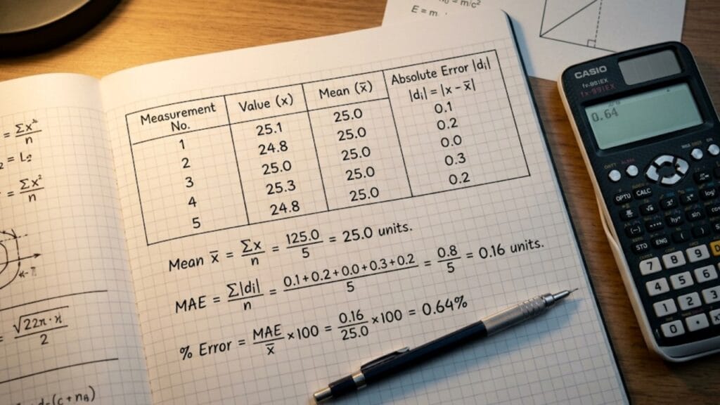
Fully Worked Example
Problem: A student measures the diameter of a wire five times using a screw gauge. The readings are: 1.23, 1.25, 1.24, 1.27 and 1.21 mm. Find (a) the mean diameter, (b) the absolute error of each reading, (c) the mean absolute error, (d) the result with uncertainty, (e) the relative error and (f) the percentage error.
Step 1: Record Measurements
\[ x_1 = 1.23, \quad x_2 = 1.25, \quad x_3 = 1.24, \quad x_4 = 1.27, \quad x_5 = 1.21 \text{ mm} \]
Step 2: Mean Value
\[ \bar{x} = \frac{1.23 + 1.25 + 1.24 + 1.27 + 1.21}{5} = \frac{6.20}{5} = 1.24 \text{ mm} \]
Step 3: Absolute Errors
\[ \Delta x_1 = |1.23 – 1.24| = 0.01 \text{ mm} \] \[ \Delta x_2 = |1.25 – 1.24| = 0.01 \text{ mm} \] \[ \Delta x_3 = |1.24 – 1.24| = 0.00 \text{ mm} \] \[ \Delta x_4 = |1.27 – 1.24| = 0.03 \text{ mm} \] \[ \Delta x_5 = |1.21 – 1.24| = 0.03 \text{ mm} \]
Step 4: Mean Absolute Error
\[ \overline{\Delta x} = \frac{0.01 + 0.01 + 0.00 + 0.03 + 0.03}{5} = \frac{0.08}{5} = 0.016 \approx 0.02 \text{ mm} \]
(Rounded to the same decimal place as the least count of the instrument, which is 0.01 mm for a standard screw gauge.)
Step 5: Result with Uncertainty
\[ d = 1.24 \pm 0.02 \text{ mm} \]
Step 6: Relative Error
\[ \delta_r = \frac{0.02}{1.24} \approx 0.016 \]
Step 7: Percentage Error
\[ \delta_\% = 0.016 \times 100\% = 1.6\% \]

Error Propagation: Carrying Errors Through Calculations
When a physical quantity is calculated from two or more measured values, the errors in those measurements propagate into the calculated result. The rules depend on the mathematical operation.
Addition and Subtraction
For \( Z = A + B \) or \( Z = A – B \):
\[ \Delta Z = \Delta A + \Delta B \]
Absolute errors add, always. Even in subtraction, errors are not subtracted — the worst-case deviation of \( Z \) from its true value occurs when both \( A \) and \( B \) deviate in the same direction.
Example: Two lengths \( A = 5.0 \pm 0.2 \) cm and \( B = 3.0 \pm 0.1 \) cm are measured. Their sum:
\[ Z = 8.0 \text{ cm}, \quad \Delta Z = 0.2 + 0.1 = 0.3 \text{ cm} \]
\[ Z = 8.0 \pm 0.3 \text{ cm} \]
Multiplication and Division
For \( Z = AB \) or \( Z = A/B \):
\[ \frac{\Delta Z}{Z} = \frac{\Delta A}{A} + \frac{\Delta B}{B} \]
Relative errors add for products and quotients.
Example: Velocity \( v = d/t \) where \( d = 10.0 \pm 0.2 \) m and \( t = 2.0 \pm 0.1 \) s:
\[ v = \frac{10.0}{2.0} = 5.0 \text{ m/s} \]
\[ \frac{\Delta v}{v} = \frac{0.2}{10.0} + \frac{0.1}{2.0} = 0.02 + 0.05 = 0.07 \]
\[ \Delta v = 0.07 \times 5.0 = 0.35 \approx 0.4 \text{ m/s} \]
\[ v = 5.0 \pm 0.4 \text{ m/s}, \quad \% \text{ error} = 7\% \]
Powers
For \( Z = A^n \):
\[ \frac{\Delta Z}{Z} = |n| \cdot \frac{\Delta A}{A} \]
The relative error is multiplied by the magnitude of the exponent. This is why errors in volume (which scales as \( r^3 \)) are three times larger in relative terms than errors in radius.
Example: Volume of a sphere \( V = \frac{4}{3}\pi r^3 \) where \( r = 5.0 \pm 0.1 \) cm:
\[ \frac{\Delta V}{V} = 3 \times \frac{\Delta r}{r} = 3 \times \frac{0.1}{5.0} = 3 \times 0.02 = 0.06 = 6\% \]
A 2% error in radius produces a 6% error in volume.
General Formula
For \( Z = \frac{A^p \cdot B^q}{C^r} \):
\[ \frac{\Delta Z}{Z} = p\frac{\Delta A}{A} + q\frac{\Delta B}{B} + r\frac{\Delta C}{C} \]
All exponents are taken as positive values. A quantity in the denominator raised to power \( r \) still contributes \( +r \cdot \frac{\Delta C}{C} \) to the relative error.
Worked Examples on Error Propagation
Example 1: Percentage Error in Kinetic Energy
The kinetic energy is \( KE = \frac{1}{2}mv^2 \). If the percentage error in mass \( m \) is 2% and in velocity \( v \) is 3%, find the percentage error in \( KE \).
Solution:
\[ \frac{\Delta KE}{KE} \times 100 = \frac{\Delta m}{m} \times 100 + 2 \times \frac{\Delta v}{v} \times 100 \]
\[ = 2\% + 2 \times 3\% = 2\% + 6\% = 8\% \]
Example 2: Percentage Error in Gravitational Acceleration
From the pendulum formula \( T = 2\pi\sqrt{L/g} \), rearranged as \( g = 4\pi^2 L / T^2 \). If the percentage error in \( L \) is 1.5% and in \( T \) is 2%, find the percentage error in \( g \).
Solution:
\[ \frac{\Delta g}{g} \times 100 = \frac{\Delta L}{L} \times 100 + 2 \times \frac{\Delta T}{T} \times 100 \]
\[ = 1.5\% + 2 \times 2\% = 1.5\% + 4\% = 5.5\% \]
Example 3: Percentage Error in Density
The density \( \rho = m/V \). Mass \( m = 50.0 \pm 0.5 \) g, Volume \( V = 25.0 \pm 0.3 \) cm³.
Solution:
\[ \rho = \frac{50.0}{25.0} = 2.0 \text{ g/cm}^3 \]
\[ \frac{\Delta\rho}{\rho} = \frac{\Delta m}{m} + \frac{\Delta V}{V} = \frac{0.5}{50.0} + \frac{0.3}{25.0} = 0.01 + 0.012 = 0.022 \]
\[ \Delta\rho = 0.022 \times 2.0 = 0.044 \approx 0.04 \text{ g/cm}^3 \]
\[ \rho = 2.00 \pm 0.04 \text{ g/cm}^3, \quad \% \text{ error} = 2.2\% \]
Example 4: Young’s Modulus Error
Young’s modulus is given by \( Y = \frac{FL}{A\Delta l} \). The percentage errors in \( F \), \( L \), \( A \) and \( \Delta l \) are 1%, 1%, 2% and 4% respectively.
Solution:
\[ \frac{\Delta Y}{Y} \times 100 = 1\% + 1\% + 2\% + 4\% = 8\% \]

Comparison: Absolute, Relative and Percentage Error
| Property | Absolute Error | Relative Error | Percentage Error |
| Symbol | \( \overline{\Delta x} \) | \( \delta_r \) | \( \delta_\% \) |
| Formula | \( \frac{\sum \Delta x_i}{n} \) | \( \frac{\overline{\Delta x}}{\bar{x}} \) | \( \frac{\overline{\Delta x}}{\bar{x}} \times 100\% \) |
| Unit | Same as measured quantity | Dimensionless | % (dimensionless) |
| Answers | “Wrong by how much?” | “Wrong by what fraction?” | “Wrong by what percent?” |
| Best used for | Result reporting, propagation of sums | Comparing precision, propagation of products | Exam answers, lab reports |
| Changes with unit? | Yes | No | No |
| Typical magnitude | Depends on quantity | 0.001 to 0.1 | 0.1% to 10% |
Common Mistakes in Error Calculations
Mistake 1: Taking the Signed Difference Instead of the Absolute Value
Absolute error is defined as \( |x_i – \bar{x}| \). The absolute value sign is essential. If a reading is below the mean, the signed difference is negative — but the error is not negative. Error is always positive. Taking the signed difference and then averaging produces a result close to zero for a symmetric distribution of errors, which is meaningless.
Mistake 2: Rounding the Mean Too Early
The mean must be calculated with sufficient decimal places before computing individual absolute errors. Rounding the mean prematurely shifts the absolute error values and corrupts the mean absolute error. Always carry at least one extra decimal place through intermediate steps and round only the final reported result.
Mistake 3: Forgetting the Absolute Value of the Exponent in Propagation
In the power rule \( \frac{\Delta Z}{Z} = |n| \cdot \frac{\Delta A}{A} \), the exponent must be taken as a positive number. If \( Z = A^{-2} \) (as occurs when \( g \propto T^{-2} \)), the contribution to relative error is still \( 2 \cdot \frac{\Delta A}{A} \), not \( -2 \cdot \frac{\Delta A}{A} \). Errors are always additive.
Mistake 4: Adding Relative Errors for Sums
The addition rule for sums (\( \Delta Z = \Delta A + \Delta B \)) uses absolute errors. The multiplication rule uses relative errors. Students frequently mix these up — applying the relative error rule to an addition problem or the absolute error rule to a multiplication problem.
Rule: Look at the mathematical operation first.
- Adding or subtracting quantities → absolute errors add
- Multiplying or dividing quantities → relative errors add
Mistake 5: Reporting More Significant Figures in the Error Than in the Mean
The mean absolute error should be rounded to the same number of significant figures as the least count of the instrument (typically one or two significant figures). The mean value is then rounded to match the decimal place of the error. Reporting \( d = 1.2400 \pm 0.0163 \) mm is incorrect — the error has too many significant figures and the mean has too many decimal places relative to the error.
Correct form: \( d = 1.24 \pm 0.02 \) mm.
[Learn more about How to Find Significant Figures: Rules, Examples & Common Mistakes]
Error in the Context of Accuracy and Precision
The three error expressions connect directly to the accuracy-precision distinction:
Absolute error and percentage error quantify accuracy — how close the measurement result is to the true value. A small percentage error means the measurement is close to the accepted value.
Mean absolute error quantifies precision — how tightly the individual readings cluster around their mean. A small mean absolute error means the measurements are reproducible.
Both are needed for a complete assessment of measurement quality. A result can have low mean absolute error (high precision, tight clustering) but high percentage error from true value (low accuracy, systematic bias). A result can have high mean absolute error (low precision, scattered readings) but low percentage error from true value (high accuracy on average).
[Learn more about Accuracy vs Precision in Physics: Definition, Difference & Real-World Examples]
[Learn more about Top 5 Errors in Physics Measurements and How to Minimize Them]
Errors in Exam Context
CBSE Board Exams
Error analysis appears in two forms:
Descriptive questions (2–3 marks): Define absolute error. Distinguish between relative error and percentage error. State the formula for mean absolute error.
Numerical questions (3 marks): Given five readings of a physical quantity, find the mean, absolute errors, mean absolute error, relative error and percentage error. Present the result in standard form.
JEE Main and NEET
Error propagation numericals are the primary format:
- Given a formula with three or four variables and their percentage errors, find the percentage error in the derived quantity.
- Given specific readings and instrument specifications, calculate the total error in a measured or derived quantity.
The general propagation formula \( \frac{\Delta Z}{Z} = p\frac{\Delta A}{A} + q\frac{\Delta B}{B} + r\frac{\Delta C}{C} \) covers every competitive exam error propagation question.
[Learn more about Units and Measurements for JEE Main: Important Topics, Formulas & PYQs]
[Learn more about NEET Physics: Units & Measurements – Chapter Notes with MCQs]
Summary: All Formulas in One Place
Basic Error Formulas
\[ \bar{x} = \frac{\sum x_i}{n} \quad \text{(Mean)} \]
\[ \Delta x_i = |x_i – \bar{x}| \quad \text{(Absolute error of } i\text{th reading)} \]
\[ \overline{\Delta x} = \frac{\sum \Delta x_i}{n} \quad \text{(Mean absolute error)} \]
\[ x = \bar{x} \pm \overline{\Delta x} \quad \text{(Result with uncertainty)} \]
\[ \delta_r = \frac{\overline{\Delta x}}{\bar{x}} \quad \text{(Relative error)} \]
\[ \delta_\% = \frac{\overline{\Delta x}}{\bar{x}} \times 100\% \quad \text{(Percentage error)} \]
Error Propagation Formulas
\[ Z = A \pm B \Rightarrow \Delta Z = \Delta A + \Delta B \]
\[ Z = AB \text{ or } \frac{A}{B} \Rightarrow \frac{\Delta Z}{Z} = \frac{\Delta A}{A} + \frac{\Delta B}{B} \]
\[ Z = A^n \Rightarrow \frac{\Delta Z}{Z} = |n| \cdot \frac{\Delta A}{A} \]
\[ Z = \frac{A^p B^q}{C^r} \Rightarrow \frac{\Delta Z}{Z} = p\frac{\Delta A}{A} + q\frac{\Delta B}{B} + r\frac{\Delta C}{C} \]
Conclusion
Absolute error, relative error and percentage error are not three separate concepts to be learned in isolation. They are three representations of the same underlying quantity — measurement uncertainty — each with its own purpose and its own place in the analysis.
Absolute error belongs in the result statement and in the propagation of sums. Relative error belongs in propagation of products and quotients. Percentage error belongs in the final report, in exam answers and in any communication where clarity and interpretability matter most.
The progression from a raw set of repeated measurements to a properly reported result with percentage error — following the seven steps of the calculation — is one of the most fundamental practical skills in experimental physics. Practice it on real data, not just example problems. Take five readings of something you can measure, compute the full chain from mean to percentage error and check your arithmetic. The procedure will become automatic faster than you expect.
[Learn more about Measurement Uncertainty in Physics: What It Is and Why It Always Exists]
[Learn more about Most Important Formulas in Units & Measurements for Board Exams]
Frequently Asked Questions
What is the difference between absolute error and mean absolute error?
Absolute error (\( \Delta x_i = |x_i – \bar{x}| \)) is the deviation of a single measurement from the mean. It is calculated separately for each reading. Mean absolute error (\( \overline{\Delta x} \)) is the average of all individual absolute errors. It represents the overall uncertainty of the measurement process and is what appears in the final result statement \( x = \bar{x} \pm \overline{\Delta x} \).
Why is absolute error always positive?
Because error represents the magnitude of uncertainty — how far off a measurement might be — not the direction. Whether a reading is above or below the mean, the error is the distance from the mean, which is always positive. Using the absolute value \( |x_i – \bar{x}| \) ensures this. A “negative error” would be physically meaningless — you cannot have a negative uncertainty.
What is relative error and when should I use it?
Relative error is the ratio of the mean absolute error to the mean value: \( \delta_r = \overline{\Delta x}/\bar{x} \). Use it when comparing the precision of measurements of different quantities or in different units and when applying error propagation rules to products and quotients. Relative error is dimensionless, so it allows meaningful comparison across different types of measurements.
How do I calculate percentage error from a set of measurements?
Follow the seven-step process: (1) list all measurements, (2) compute the mean, (3) compute the absolute error of each reading, (4) compute the mean absolute error, (5) report the result as mean ± mean absolute error, (6) divide mean absolute error by the mean to get relative error, (7) multiply by 100 to get percentage error.
What is the percentage error formula when comparing to an accepted value?
When a true or accepted value is known, percentage error is calculated as: \( \frac{|\text{Measured} – \text{Accepted}|}{\text{Accepted}} \times 100\% \). This measures how far the experimental result is from the known standard — it is a measure of accuracy. This is different from the percentage error calculated from repeated measurements, which measures precision.
Why do errors always add in subtraction?
The rule \( \Delta Z = \Delta A + \Delta B \) applies to both addition and subtraction because errors represent the worst-case scenario. When computing \( Z = A – B \), the maximum possible deviation of \( Z \) from its true value occurs when \( A \) is at its maximum (\( \bar{A} + \Delta A \)) and \( B \) is at its minimum (\( \bar{B} – \Delta B \)), or vice versa. In either case, the total deviation in \( Z \) is \( \Delta A + \Delta B \). The sign of the arithmetic operation does not change this.
Leave a Comment