

Introduction
A measurement is never the end of the story. In most experiments, the quantity you actually want cannot be measured directly — it must be calculated from two or more directly measured quantities. You might measure the length and time of fall to find gravitational acceleration. You might measure mass and volume to find density. You might measure voltage and current to find resistance.
Each of those measured quantities carries an error. When you combine them through a formula, those individual errors combine too — they propagate into the calculated result. The result carries an error of its own and that error is determined by the errors in the inputs and by the mathematical structure of the formula.
Understanding how errors propagate is not optional for anyone doing experimental physics. It determines how many significant figures your result deserves, which measurement you should improve to get the biggest gain in precision and whether your result is consistent with the accepted value. This article covers every propagation rule with full derivations of reasoning, all formulas and enough worked examples to make the application mechanical under exam conditions.
What Is Error Propagation?
When a derived quantity \( Z \) is calculated from measured quantities \( A \), \( B \), \( C \), \ldots, each of which has its own uncertainty, the uncertainty in \( Z \) depends on:
- The uncertainties in \( A \), \( B \), \( C \), \ldots
- The mathematical relationship \( Z = f(A, B, C, \ldots) \)
Error propagation is the process of determining the uncertainty in \( Z \) from the uncertainties in its inputs, given the functional relationship between them.
The core physical reasoning: an error in \( A \) by \( \Delta A \) causes a change in \( Z \). The size of that change depends on how sensitively \( Z \) responds to \( A \) — which is determined by the partial derivative \( \partial Z / \partial A \), or equivalently by the structure of the formula. Each input contributes its own error to the output and in the worst case, all contributions act in the same direction. This worst-case analysis gives the maximum possible error in \( Z \).
The General Formula: Partial Derivatives Approach
For a general function \( Z = f(A, B, C) \), the maximum absolute error in \( Z \) is:
\[ \Delta Z = \left|\frac{\partial Z}{\partial A}\right| \Delta A + \left|\frac{\partial Z}{\partial B}\right| \Delta B + \left|\frac{\partial Z}{\partial C}\right| \Delta C \]
This is the full mathematical statement of error propagation. Every specific rule we derive below is a special case of this formula applied to a particular functional form.
The absolute value signs around each partial derivative are essential — they ensure all contributions are positive (worst-case, all errors add rather than cancelling).
In practice, for the functional forms common in physics (sums, products, powers), the partial derivative approach simplifies to a small set of clean rules that do not require explicit calculus. These rules are what appear in CBSE board exams, JEE Main and NEET.
Rule 1: Error in a Sum or Difference
Formula
For \( Z = A + B \) or \( Z = A – B \):
\[ \Delta Z = \Delta A + \Delta B \]
Absolute errors always add, regardless of whether the operation is addition or subtraction.
Derivation
For \( Z = A + B \):
\[ \frac{\partial Z}{\partial A} = 1, \quad \frac{\partial Z}{\partial B} = 1 \]
\[ \Delta Z = |1| \cdot \Delta A + |1| \cdot \Delta B = \Delta A + \Delta B \]
For \( Z = A – B \):
\[ \frac{\partial Z}{\partial A} = 1, \quad \frac{\partial Z}{\partial B} = -1 \]
\[ \Delta Z = |1| \cdot \Delta A + |-1| \cdot \Delta B = \Delta A + \Delta B \]
The result is the same. The sign of the operation does not affect how errors combine.
Physical Reasoning
When you subtract \( B \) from \( A \), the worst case is when \( A \) is at its maximum possible value and \( B \) is at its minimum possible value — or vice versa. In either scenario, the deviation of \( Z \) from its true value is \( \Delta A + \Delta B \). The subtraction brings the measurements closer together, but the uncertainty in the result is larger, not smaller.
Example
A metal rod is cut from a bar. The bar length is \( L_1 = 120.5 \pm 0.2 \) cm. The remaining piece is \( L_2 = 84.3 \pm 0.2 \) cm. The cut piece length:
\[ L = L_1 – L_2 = 36.2 \text{ cm} \]
\[ \Delta L = \Delta L_1 + \Delta L_2 = 0.2 + 0.2 = 0.4 \text{ cm} \]
\[ L = 36.2 \pm 0.4 \text{ cm} \]
Note: the percentage error in \( L \) is \( 0.4/36.2 \times 100\% = 1.1\% \), which is much larger than the percentage error in either original measurement (\( 0.2/120.5 = 0.17\% \) and \( 0.2/84.3 = 0.24\% \)). Subtraction amplifies relative error — a critical practical point. Taking the small difference between two large, nearly equal quantities is one of the most error-prone operations in experimental physics.
Rule 2: Error in a Product or Quotient
Formula
For \( Z = A \times B \) or \( Z = A / B \):
\[ \frac{\Delta Z}{Z} = \frac{\Delta A}{A} + \frac{\Delta B}{B} \]
Relative errors add for products and quotients.
Derivation for Product
\( Z = AB \)
\[ \frac{\partial Z}{\partial A} = B, \quad \frac{\partial Z}{\partial B} = A \]
\[ \Delta Z = |B| \cdot \Delta A + |A| \cdot \Delta B \]
Dividing both sides by \( Z = AB \):
\[ \frac{\Delta Z}{Z} = \frac{\Delta A}{A} + \frac{\Delta B}{B} \]
Derivation for Quotient
\( Z = A/B \)
\[ \frac{\partial Z}{\partial A} = \frac{1}{B}, \quad \frac{\partial Z}{\partial B} = -\frac{A}{B^2} \]
\[ \Delta Z = \frac{\Delta A}{B} + \frac{A}{B^2}\Delta B \]
Dividing by \( Z = A/B \):
\[ \frac{\Delta Z}{Z} = \frac{\Delta A}{A} + \frac{\Delta B}{B} \]
Same result for both operations.
Example
Velocity is calculated from \( v = d/t \) where \( d = 15.0 \pm 0.3 \) m and \( t = 3.0 \pm 0.1 \) s.
\[ v = \frac{15.0}{3.0} = 5.0 \text{ m/s} \]
\[ \frac{\Delta v}{v} = \frac{\Delta d}{d} + \frac{\Delta t}{t} = \frac{0.3}{15.0} + \frac{0.1}{3.0} = 0.02 + 0.0\overline{3} = 0.053\overline{3} \]
\[ \Delta v = 0.053\overline{3} \times 5.0 \approx 0.27 \text{ m/s} \approx 0.3 \text{ m/s} \]
\[ v = 5.0 \pm 0.3 \text{ m/s}, \quad \% \text{ error} = 5.3\% \]
Rule 3: Error in a Power
Formula
For \( Z = A^n \) (where \( n \) is any real number, positive or negative):
\[ \frac{\Delta Z}{Z} = |n| \cdot \frac{\Delta A}{A} \]
The relative error is multiplied by the absolute value of the exponent.
Derivation
\[ Z = A^n \Rightarrow \frac{dZ}{dA} = nA^{n-1} \]
\[ \Delta Z = |nA^{n-1}| \cdot \Delta A \]
\[ \frac{\Delta Z}{Z} = \frac{|nA^{n-1}| \cdot \Delta A}{A^n} = |n| \cdot \frac{\Delta A}{A} \]
The absolute value of \( n \) appears because error is always positive regardless of the sign of the exponent.
Critical Implication
When a measured quantity appears raised to a power \( n \), its contribution to the relative error of the result is amplified by a factor of \( |n| \). This means:
- An error in a squared quantity contributes twice as much to the relative error as the same fractional error in a linear quantity
- An error in a cubed quantity contributes three times as much
- An error in a square root quantity contributes half as much
This has direct practical consequences for experiment design: if your formula contains \( r^3 \), improving the measurement of \( r \) gives three times the reduction in final error compared to improving a linear factor.
Example
Volume of a sphere: \( V = \frac{4}{3}\pi r^3 \). Radius \( r = 3.50 \pm 0.02 \) cm.
\[ \frac{\Delta V}{V} = 3 \times \frac{\Delta r}{r} = 3 \times \frac{0.02}{3.50} = 3 \times 0.00571 = 0.01714 \]
\[ \% \text{ error in } V = 1.71\% \]
\[ V = \frac{4}{3}\pi (3.50)^3 = \frac{4}{3}\pi \times 42.875 \approx 179.6 \text{ cm}^3 \]
\[ \Delta V = 0.01714 \times 179.6 \approx 3.1 \text{ cm}^3 \]
\[ V = 179.6 \pm 3.1 \text{ cm}^3 \]
A 0.57% error in radius becomes a 1.71% error in volume — exactly tripled by the cube power.
Rule 4: The General Formula
Formula
For any combination of products, quotients and powers:
\[ Z = \frac{A^p \cdot B^q}{C^r} \]
\[ \frac{\Delta Z}{Z} = p\frac{\Delta A}{A} + q\frac{\Delta B}{B} + r\frac{\Delta C}{C} \]
All exponents are taken as positive. A quantity in the denominator raised to power \( r \) still contributes \( +r \cdot \frac{\Delta C}{C} \) to the relative error — never subtracted.
Derivation
Taking the natural logarithm of both sides:
\[ \ln Z = p\ln A + q\ln B – r\ln C \]
Differentiating (treating differentials as small uncertainties):
\[ \frac{dZ}{Z} = p\frac{dA}{A} + q\frac{dB}{B} – r\frac{dC}{C} \]
For maximum error, all terms are taken positive:
\[ \frac{\Delta Z}{Z} = p\frac{\Delta A}{A} + q\frac{\Delta B}{B} + r\frac{\Delta C}{C} \]
This logarithmic differentiation method is elegant and extends to any number of variables with any combination of powers.
Extended General Formula
For any formula \( Z = \frac{A^p \cdot B^q \cdot D^s}{C^r \cdot E^t} \):
\[ \frac{\Delta Z}{Z} = p\frac{\Delta A}{A} + q\frac{\Delta B}{B} + s\frac{\Delta D}{D} + r\frac{\Delta C}{C} + t\frac{\Delta E}{E} \]
Every variable in the formula contributes its relative error multiplied by the absolute value of its power.
Summary: All Four Rules Side by Side
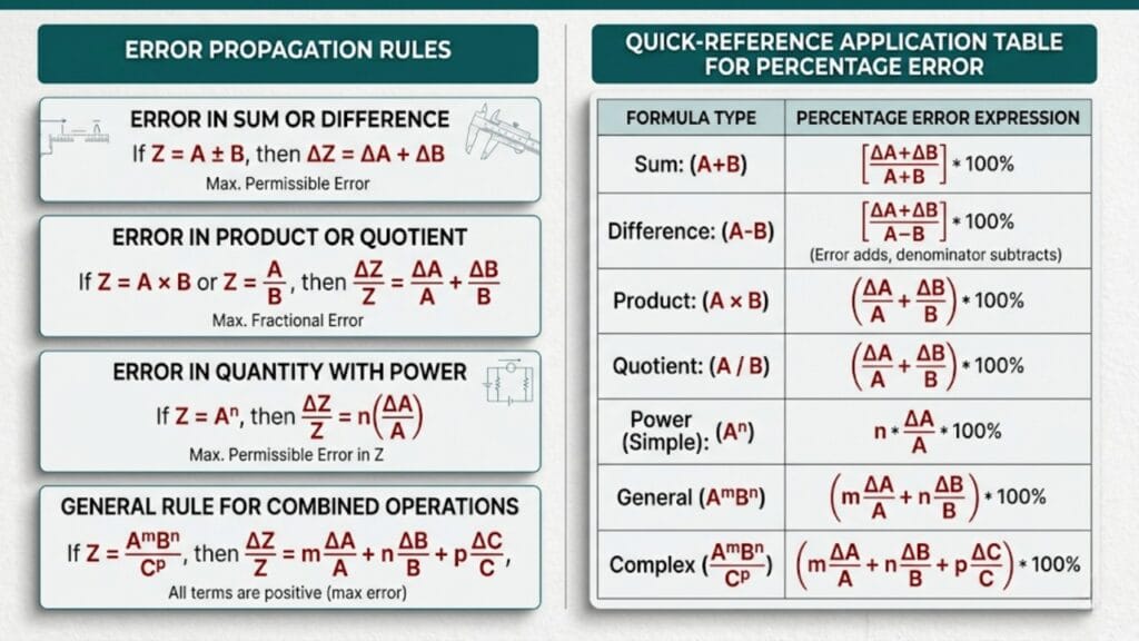
| Operation | Formula | Uses |
| \( Z = A + B \) or \( Z = A – B \) | \( \Delta Z = \Delta A + \Delta B \) | Absolute errors add |
| \( Z = AB \) or \( Z = A/B \) | \( \frac{\Delta Z}{Z} = \frac{\Delta A}{A} + \frac{\Delta B}{B} \) | Relative errors add |
| \( Z = A^n \) | \( \frac{\Delta Z}{Z} = \|n\| \cdot \frac{\Delta A}{A} \) | Exponent multiplies relative error |
| \( Z = \frac{A^p B^q}{C^r} \) | \( \frac{\Delta Z}{Z} = p\frac{\Delta A}{A} + q\frac{\Delta B}{B} + r\frac{\Delta C}{C} \) | General case — all positive |
Worked Examples
These examples progress from direct application to multi-step problems of the type appearing in board exams and JEE/NEET.
Example 1: Resistance from Ohm’s Law
Problem: In an experiment, \( V = 10.0 \pm 0.2 \) V and \( I = 2.50 \pm 0.05 \) A. Find the resistance \( R = V/I \) and its percentage error.
Solution:
\[ R = \frac{10.0}{2.50} = 4.00 \text{ Ω} \]
\[ \frac{\Delta R}{R} = \frac{\Delta V}{V} + \frac{\Delta I}{I} = \frac{0.2}{10.0} + \frac{0.05}{2.50} = 0.02 + 0.02 = 0.04 \]
\[ \% \text{ error in } R = 4\% \]
\[ \Delta R = 0.04 \times 4.00 = 0.16 \approx 0.2 \text{ Ω} \]
\[ R = 4.0 \pm 0.2 \text{ Ω} \]
Example 2: Gravitational Acceleration from Pendulum
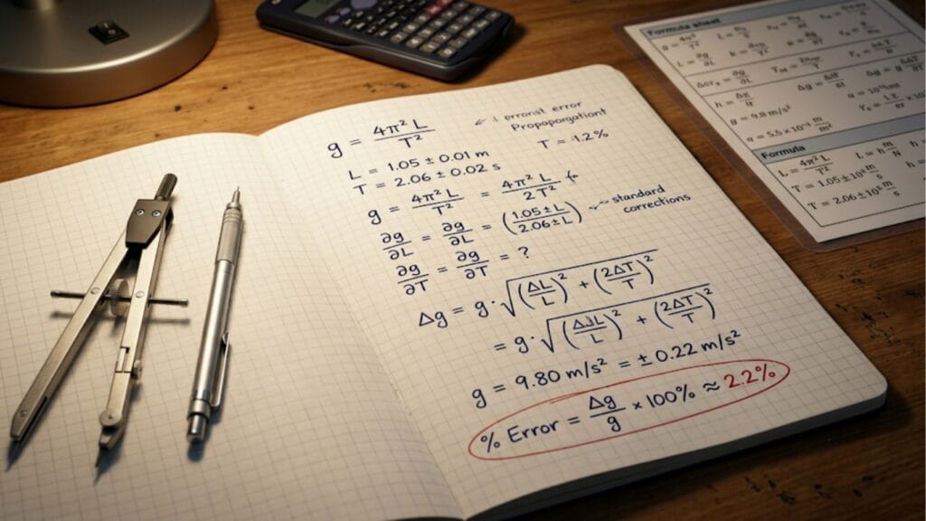
Problem: \( g = \frac{4\pi^2 L}{T^2} \). Measured: \( L = 1.000 \pm 0.005 \) m, \( T = 2.00 \pm 0.02 \) s. Find the percentage error in \( g \).
Solution:
\[ \frac{\Delta g}{g} \times 100 = \frac{\Delta L}{L} \times 100 + 2 \times \frac{\Delta T}{T} \times 100 \]
\[ = \frac{0.005}{1.000} \times 100 + 2 \times \frac{0.02}{2.00} \times 100 \]
\[ = 0.5\% + 2 \times 1\% = 0.5\% + 2\% = 2.5\% \]
Observation: The time measurement contributes \( 2\% \) while the length measurement contributes only \( 0.5\% \). To improve the overall precision, reducing the error in \( T \) would give more benefit than reducing the error in \( L \). This is how error analysis guides experimental design — it identifies the dominant error source.
Example 3: Young’s Modulus
Problem: \( Y = \frac{FL}{A\Delta l} \). Percentage errors: \( F = 1\% \), \( L = 1\% \), \( A = 2\% \), \( \Delta l = 4\% \). Find the percentage error in \( Y \).
Solution:
\[ \frac{\Delta Y}{Y} \times 100 = \frac{\Delta F}{F} \times 100 + \frac{\Delta L}{L} \times 100 + \frac{\Delta A}{A} \times 100 + \frac{\Delta l}{\Delta l} \times 100 \]
\[ = 1\% + 1\% + 2\% + 4\% = 8\% \]
Observation: The elongation \( \Delta l \) contributes 4% — half the total. In a wire-stretching Young’s modulus experiment, measuring the small extension precisely is the critical challenge. This explains why the experiment uses a travelling microscope rather than a ruler for the extension measurement.
Example 4: Kinetic Energy
Problem: \( KE = \frac{1}{2}mv^2 \). Errors: \( m = 1.5\% \), \( v = 2.5\% \). Find the percentage error in \( KE \).
Solution:
The \( \frac{1}{2} \) is a dimensionless constant — it contributes zero error.
\[ \frac{\Delta KE}{KE} \times 100 = \frac{\Delta m}{m} \times 100 + 2 \times \frac{\Delta v}{v} \times 100 \]
\[ = 1.5\% + 2 \times 2.5\% = 1.5\% + 5\% = 6.5\% \]
Example 5: Density Calculation
Problem: A cylindrical object has mass \( m = 250.0 \pm 0.5 \) g, radius \( r = 2.50 \pm 0.02 \) cm and length \( l = 10.0 \pm 0.1 \) cm. The density is \( \rho = m/(\pi r^2 l) \). Find the percentage error in density.
Solution:
\[ \frac{\Delta\rho}{\rho} \times 100 = \frac{\Delta m}{m} \times 100 + 2\frac{\Delta r}{r} \times 100 + \frac{\Delta l}{l} \times 100 \]
\[ = \frac{0.5}{250.0} \times 100 + 2 \times \frac{0.02}{2.50} \times 100 + \frac{0.1}{10.0} \times 100 \]
\[ = 0.2\% + 2 \times 0.8\% + 1.0\% \]
\[ = 0.2\% + 1.6\% + 1.0\% = 2.8\% \]
Computing the density value:
\[ \rho = \frac{250.0}{\pi \times (2.50)^2 \times 10.0} = \frac{250.0}{\pi \times 62.5} = \frac{250.0}{196.35} \approx 1.273 \text{ g/cm}^3 \]
\[ \Delta\rho = 0.028 \times 1.273 \approx 0.036 \approx 0.04 \text{ g/cm}^3 \]
\[ \rho = 1.27 \pm 0.04 \text{ g/cm}^3 \]
Observation: The radius contributes \( 1.6\% \) (dominant), the length \( 1.0\% \) and the mass only \( 0.2\% \). A better caliper for the radius would help more than a better balance.
Example 6: Power Dissipation
Problem: Power dissipated is \( P = I^2 R \). If the percentage error in current \( I \) is 3% and in resistance \( R \) is 2%, find the percentage error in \( P \).
Solution:
\[ \frac{\Delta P}{P} \times 100 = 2 \times \frac{\Delta I}{I} \times 100 + \frac{\Delta R}{R} \times 100 \]
\[ = 2 \times 3\% + 2\% = 6\% + 2\% = 8\% \]
Example 7: Gravitational Force Between Two Masses
Problem: \( F = \frac{Gm_1 m_2}{r^2} \). Percentage errors: \( m_1 = 1\% \), \( m_2 = 2\% \), \( r = 1.5\% \). Find the percentage error in \( F \). (Treat \( G \) as exact.)
Solution:
\[ \frac{\Delta F}{F} \times 100 = \frac{\Delta m_1}{m_1} \times 100 + \frac{\Delta m_2}{m_2} \times 100 + 2\frac{\Delta r}{r} \times 100 \]
\[ = 1\% + 2\% + 2 \times 1.5\% = 1\% + 2\% + 3\% = 6\% \]
Example 8: The Period of a Spring-Mass System
Problem: \( T = 2\pi\sqrt{m/k} \). Percentage errors: \( m = 2\% \), \( k = 3\% \). Find the percentage error in \( T \).
Solution:
Rewrite as: \( T = 2\pi \cdot m^{1/2} \cdot k^{-1/2} \)
\[ \frac{\Delta T}{T} \times 100 = \frac{1}{2} \times \frac{\Delta m}{m} \times 100 + \frac{1}{2} \times \frac{\Delta k}{k} \times 100 \]
\[ = \frac{1}{2} \times 2\% + \frac{1}{2} \times 3\% = 1\% + 1.5\% = 2.5\% \]
Note: The square root halves the contribution of each error. The constant \( 2\pi \) is dimensionless and contributes nothing.
Special Cases and Subtleties
Dimensionless Constants Do Not Contribute
Constants like \( \frac{1}{2} \), \( 2\pi \), \( \frac{4}{3} \) and \( \pi \) are exact by definition. They carry zero error and contribute nothing to the propagated uncertainty. This is why the \( 2\pi \) in the pendulum formula and the \( \frac{1}{2} \) in the kinetic energy formula are simply ignored in error propagation.
Identical Variables Appearing Multiple Times
If the same measured quantity appears more than once in a formula, treat it as a single variable with its power equal to the combined exponent.
Example: \( Z = A \cdot A^2 = A^3 \)
\[ \frac{\Delta Z}{Z} = 3\frac{\Delta A}{A} \]
Do not add the error for \( A \) twice. The variable appears to power 3 in total.
This is important for formulas like \( P = V^2/R \):
\[ \frac{\Delta P}{P} = 2\frac{\Delta V}{V} + \frac{\Delta R}{R} \]
Not \( \frac{\Delta V}{V} + \frac{\Delta V}{V} + \frac{\Delta R}{R} \) (which would give the same answer, but the reasoning must be clear).
The Subtraction Amplification Effect
When \( Z = A – B \) and \( A \approx B \) (the two measured quantities are nearly equal), the absolute error in \( Z \) is the same as in any other subtraction (\( \Delta A + \Delta B \)). But because \( Z \) is small, the relative error becomes large.
Example: \( A = 100.0 \pm 0.5 \), \( B = 99.0 \pm 0.5 \)
\[ Z = 1.0, \quad \Delta Z = 1.0 \]
\[ \frac{\Delta Z}{Z} = 100\% \]
A relative error of 100% means the result is completely uncertain — the measurement tells you almost nothing about the true value of \( Z \). This situation, called catastrophic cancellation or loss of significance, is a major practical concern in precision measurement and numerical computing. Experimental design should avoid, where possible, computing small differences between large, nearly-equal measured quantities.
When the Independent Variable Has No Error
If a formula contains a physical constant (like \( G \), \( c \), or \( e \)) or a dimensionless mathematical constant (like \( \pi \)), those quantities are treated as having zero uncertainty. Only measured quantities with non-zero uncertainties contribute to error propagation.
Error Propagation and Significant Figures: The Connection
The result of an error propagation calculation determines how many significant figures the final answer deserves.
The general rule: the absolute error should be rounded to one or two significant figures and the result should be rounded to match the decimal place of the error.
Example: If the calculation gives \( \rho = 2.3847 \pm 0.0632 \text{ g/cm}^3 \):
- Round \( \Delta\rho \) to 2 significant figures: \( 0.063 \text{ g/cm}^3 \) → or to 1 sig fig: \( 0.06 \text{ g/cm}^3 \)
- Round \( \rho \) to match: \( 2.38 \pm 0.06 \text{ g/cm}^3 \)
Reporting \( 2.3847 \pm 0.0632 \) implies a precision of ±0.0001 in the last digit of the result — far beyond what the error estimate supports.
Learn more about How to Find Significant Figures: Rules, Examples & Common Mistakes
Error Propagation in Multi-Step Calculations
Sometimes a derived quantity feeds into another calculation. The error propagates through each step.
Problem: From a pendulum experiment:
- Measured \( L = 0.800 \pm 0.005 \) m
- Measured \( T = 1.80 \pm 0.02 \) s
Step 1: Calculate \( g = 4\pi^2 L / T^2 \)
\[ g = \frac{4\pi^2 \times 0.800}{(1.80)^2} = \frac{31.583 \times 0.800}{3.24} = \frac{25.266}{3.24} \approx 9.77 \text{ m/s}^2 \]
\[ \frac{\Delta g}{g} = \frac{\Delta L}{L} + 2\frac{\Delta T}{T} = \frac{0.005}{0.800} + 2 \times \frac{0.02}{1.80} \]
\[ = 0.00625 + 0.02222 = 0.02847 \approx 2.85\% \]
\[ \Delta g = 0.02847 \times 9.77 \approx 0.28 \text{ m/s}^2 \]
\[ g = 9.77 \pm 0.28 \text{ m/s}^2 \]
Step 2: Does the result agree with the accepted value \( g = 9.81 \) m/s²?
The measured result spans \( [9.49, 10.05] \) m/s². The accepted value \( 9.81 \) lies within this range. The measurement is consistent with the accepted value at the stated precision level.
This is the physical meaning of error analysis — checking whether your result is consistent with known physics, or whether the discrepancy is large enough to require explanation.
Common Mistakes in Error Propagation
Mistake 1: Subtracting Errors for a Difference
\( \Delta Z = \Delta A + \Delta B \) always — for both \( Z = A + B \) and \( Z = A – B \). Never \( \Delta A – \Delta B \). This mistake arises from the intuition that subtraction reduces the result, so it should reduce the error. The error analysis considers the worst case, where the errors act in opposite directions and both increase the deviation.
Mistake 2: Using Absolute Instead of Relative Errors for Products
For \( Z = AB \), the correct formula is \( \frac{\Delta Z}{Z} = \frac{\Delta A}{A} + \frac{\Delta B}{B} \) (relative errors). Writing \( \Delta Z = \Delta A + \Delta B \) (absolute errors) is wrong for multiplication — it applies only to addition and subtraction.
The mnemonic: identify the operation first, then choose the rule.
Mistake 3: Forgetting the Exponent in the Power Rule
In \( Z = A^n \), the formula is \( \frac{\Delta Z}{Z} = |n| \cdot \frac{\Delta A}{A} \). The \( |n| \) factor is the most commonly omitted step. Particularly in the pendulum formula, where \( g \propto T^{-2} \), students often write \( \frac{\Delta g}{g} = \frac{\Delta T}{T} \) instead of \( 2\frac{\Delta T}{T} \).
Mistake 4: Treating a Physical Constant as Having Error
\( G \), \( c \), \( e \) and \( \pi \) are either exact or treated as having negligible uncertainty relative to experimental measurements. Including them in error propagation adds nothing and confuses the calculation.
Mistake 5: Not Reporting to Appropriate Significant Figures
After computing the percentage error and the absolute error, the final result must be rounded to match the decimal place of the error. Keeping five decimal places in the result while the error is known to two significant figures is misleading overclaiming.
Learn more about Absolute Error, Relative Error and Percentage Error: A Complete Guide
Error Propagation in Exam Context
CBSE Board Exams
Error propagation appears as 3-mark numerical questions. The typical format:
“Given \( Z = A^2 B / \sqrt{C} \), with percentage errors 2%, 3%, 4% in A, B, C respectively, find the percentage error in Z.”
Apply the general formula directly:
\[ \frac{\Delta Z}{Z} \times 100 = 2(2\%) + 3\% + \frac{1}{2}(4\%) = 4\% + 3\% + 2\% = 9\% \]
JEE Main and NEET
These exams test error propagation in two ways:
- Direct formula questions: Percentage error in a derived quantity given percentage errors in measured quantities.
- Instrument-based questions: Given the least count of instruments used to measure physical quantities in a formula, find the minimum possible percentage error in the derived quantity.
For Type 2, the minimum error per measurement is the instrument’s least count and this propagates through the formula exactly as a measured error would.
Learn more about Units and Measurements for JEE Main: Important Topics, Formulas & PYQs
Learn more about NEET Physics: Units & Measurements – Chapter Notes with MCQs
Quick Reference: Error Propagation in Common Physics Formulas
| Formula | % Error Expression |
| \( v = d/t \) | \( \%v = \%d + \%t \) |
| \( KE = \frac{1}{2}mv^2 \) | \( \%KE = \%m + 2(\%v) \) |
| \( g = 4\pi^2 L/T^2 \) | \( \%g = \%L + 2(\%T) \) |
| \( \rho = m/V \) | \( \%\rho = \%m + \%V \) |
| \( \rho_\text{cylinder} = m/(\pi r^2 l) \) | \( \%\rho = \%m + 2(\%r) + \%l \) |
| \( R = V/I \) | \( \%R = \%V + \%I \) |
| \( P = I^2 R \) | \( \%P = 2(\%I) + \%R \) |
| \( P = V^2/R \) | \( \%P = 2(\%V) + \%R \) |
| \( F = GMm/r^2 \) | \( \%F = \%M + \%m + 2(\%r) \) |
| \( T = 2\pi\sqrt{L/g} \) | \( \%T = \frac{1}{2}(\%L) + \frac{1}{2}(\%g) \) |
| \( V_\text{sphere} = \frac{4}{3}\pi r^3 \) | \( \%V = 3(\%r) \) |
| \( Y = FL/(A\Delta l) \) | \( \%Y = \%F + \%L + \%A + \%(\Delta l) \) |
Conclusion
Error propagation is the logical completion of any experimental measurement. A measurement without an uncertainty statement is incomplete; a derived quantity without propagated error is doubly incomplete — it conceals not just the uncertainty in the final result but the contributions of each individual measurement.
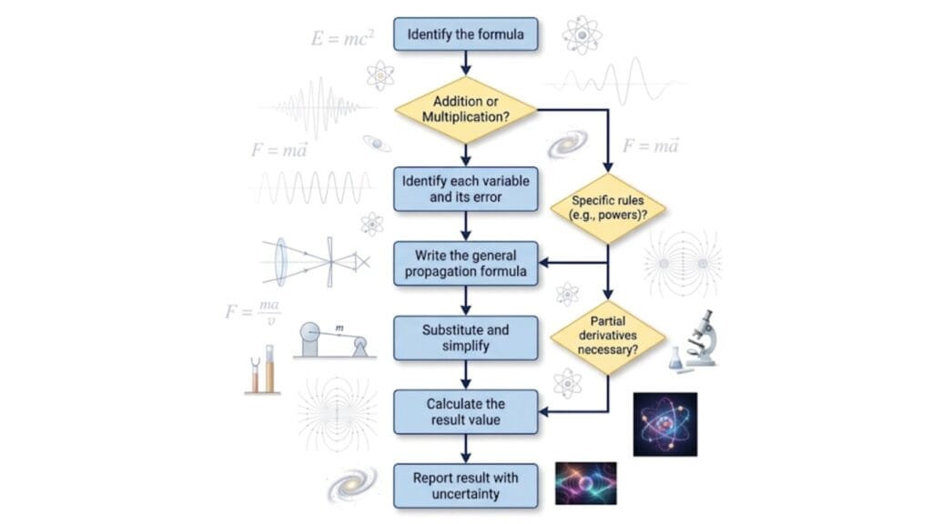
The four rules covered in this article — sum/difference, product/quotient, power and general — are all special cases of a single underlying principle: the maximum error in a derived quantity is the sum of the absolute values of the partial derivative contributions from each input. The rules emerge naturally from this principle and once you see where they come from, they are impossible to forget in the ways that memorized rules always are.
The practical skill is applying them quickly and correctly. Work through the examples in this article on paper — substituting your own numbers if it helps. Make the process automatic. When you sit down in an exam with a formula you have never seen before, you will be able to write down the error propagation expression immediately, without hesitation, because the logic is always the same.
Learn more about Measurement Uncertainty in Physics: What It Is and Why It Always Exists
Frequently Asked Questions
Why do errors always add in subtraction?
Because error propagation uses the worst-case scenario. When computing \( Z = A – B \), the maximum possible deviation from the true value of \( Z \) occurs when \( A \) is at its maximum and \( B \) is at its minimum, or vice versa. In both cases, the deviation is \( \Delta A + \Delta B \). The sign of the arithmetic operation cannot help — it cannot make the errors cancel.
What is the difference between absolute error and relative error in propagation?
Absolute error (\( \Delta Z \)) is used in the sum/difference rule and carries the same unit as the measured quantity. Relative error (\( \Delta Z / Z \)) is dimensionless and is used in the product/quotient and power rules. In practice, percentage error (relative error × 100%) is the most commonly quoted form.
Does a physical constant like \( G \) or \( \pi \) contribute to error propagation?
No. Physical constants and exact mathematical constants have zero uncertainty by definition and contribute nothing to error propagation. Only measured quantities with non-zero uncertainties contribute.
How do I find the dominant error source in an experiment?
Calculate the individual contributions of each measured quantity to the total percentage error. The term that contributes the largest percentage is the dominant source. Improving the precision of the dominant source gives the largest reduction in total error — this is how error analysis guides experimental design.
What happens to error when I take a square root?
The power rule applies: for \( Z = A^{1/2} \), the relative error in \( Z \) is \( \frac{1}{2} \cdot \frac{\Delta A}{A} \). The square root halves the relative error contribution from \( A \). This is why the pendulum formula \( T = 2\pi\sqrt{L/g} \) has the \( \frac{1}{2} \) factor on both \( \%L \) and \( \%g \) when computing \( \%T \).
Can percentage errors exceed 100%?
Yes. This happens when the subtraction of two nearly equal quantities gives a very small result — a phenomenon called catastrophic cancellation. If the absolute uncertainty in the difference is comparable to or larger than the difference itself, the relative error approaches or exceeds 100%, making the measurement essentially meaningless for the intended purpose.
How do I report the final result after error propagation?
Round the absolute error to one or two significant figures. Then round the result value to the same decimal place as the error. Report as: \( Z = \bar{Z} \pm \Delta Z \) (units). For example: \( \rho = 2.38 \pm 0.06 \text{ g/cm}^3 \).
Leave a Comment