

Introduction
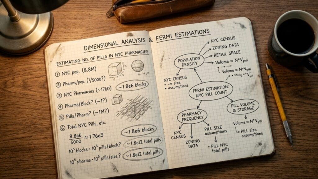
Enrico Fermi once asked his students to estimate the number of piano tuners in Chicago. He had no data. No reference books. No internet. Just a quiet pause, a few scribbled numbers on the back of an envelope and an answer: roughly 125. The actual number, when later verified against telephone directory listings, was around 100 to 150.
Fermi’s method was not guesswork. It was systematic decomposition — breaking an apparently impossible question into a chain of individually estimable steps, estimating each step to the nearest order of magnitude and multiplying through to the answer. The method is named after him today and it is one of the most practically useful reasoning tools in all of physics.
This article teaches the method from first principles, explains the underlying physics of order-of-magnitude reasoning and works through a series of problems that range from the textbook-familiar to the genuinely surprising. By the end, you will be able to estimate quantities that you have never measured, never looked up and perhaps never even thought about — with confidence, on the back of an envelope.
What Is Order of Magnitude?
Before Fermi estimation, the concept of order of magnitude needs to be precise.
The order of magnitude of a number is the power of 10 closest to that number. More precisely:
If \( N = a \times 10^n \) where \( 1 \leq a < 10 \):
\[ \text{Order of magnitude} = \begin{cases} 10^n & \text{if } a < \sqrt{10} \approx 3.162 \ 10^{n+1} & \text{if } a \geq \sqrt{10} \end{cases} \]
Examples:
- \( 4700 = 4.7 \times 10^3 \): since \( 4.7 > 3.162 \), order of magnitude is \( 10^4 \)
- \( 2100 = 2.1 \times 10^3 \): since \( 2.1 < 3.162 \), order of magnitude is \( 10^3 \)
- \( 0.0065 = 6.5 \times 10^{-3} \): since \( 6.5 > 3.162 \), order of magnitude is \( 10^{-2} \)
Why the \( \sqrt{10} \) threshold? On a logarithmic scale, the midpoint between \( 10^n \) and \( 10^{n+1} \) is \( 10^{n+1/2} = \sqrt{10} \times 10^n \). Numbers above this midpoint are geometrically closer to \( 10^{n+1} \); numbers below are closer to \( 10^n \).
In Fermi estimation, being within one order of magnitude means your answer is within a factor of 10 of the true value. Being within two orders of magnitude means within a factor of 100. For quantities that span many orders of magnitude, getting within one order is often all that is needed — and it is usually achievable.
Why Order-of-Magnitude Estimates Are Useful
A Fermi estimate is not trying to get the exact answer. It is trying to get the right scale. And knowing the right scale is often all you need.
Consider a few situations where knowing the order of magnitude matters:
Engineering feasibility: Before calculating the exact structural load of a proposed bridge, an engineer needs to know whether the loads are in the tonnes range or the megatonnes range. The feasibility of the design depends on the scale.
Scientific hypothesis testing: Before running an expensive experiment, a physicist wants to know whether the expected signal is detectable. If the signal-to-noise ratio is estimated at \( 10^{-10} \), the experiment is probably infeasible with current technology. If it is \( 10^{-2} \), it is straightforward.
Error detection: If you compute a numerical answer and it is off by three orders of magnitude from a rough estimate, something has gone wrong. Fermi estimation acts as a sanity check on detailed calculations.
Communication: Explaining that the national debt is roughly \( 10^{13} \) dollars is clearer in many contexts than saying $9.87 trillion — especially when comparing with a GDP of roughly \( 10^{13} \) dollars.
The Fermi Method: Step by Step
The Fermi method has a consistent structure regardless of the problem.
Step 1: Identify the unknown quantity. State clearly what you are trying to estimate. Give it a symbol if helpful.
Step 2: Decompose into factors. Break the unknown into a product (or ratio) of simpler quantities, each of which can be estimated independently.
Step 3: Estimate each factor. For each factor, use any combination of: direct knowledge, dimensional reasoning, scaling from a known comparable, or physical constraint.
Step 4: Multiply through and take the order of magnitude. Compute the product. Round each intermediate estimate to the nearest power of 10 for simplicity, or keep one significant figure and track the powers separately.
Step 5: Sanity check. Does the answer make physical sense? Is it consistent with anything you already know? If not, identify which factor is most likely wrong and revise.
Core Estimation Anchors: Numbers to Know
Fermi estimation relies on a bank of known quantities — the “anchor values” you carry in memory and use as starting points. Here are the most useful ones for physics:
| Quantity | Value | Order |
| Earth’s radius | 6400 km | \( 6.4 \times 10^6 \) m |
| Earth’s mass | \( 6 \times 10^{24} \) kg | \( 10^{24} \) kg |
| Earth’s surface area | \( 5.1 \times 10^{14} \) m² | \( 10^{14} \) m² |
| Earth’s population | \( 8 \times 10^9 \) | \( 10^{10} \) |
| Speed of light | \( 3 \times 10^8 \) m/s | \( 10^9 \) m/s |
| Proton mass | \( 1.67 \times 10^{-27} \) kg | \( 10^{-27} \) kg |
| Electron mass | \( 9.1 \times 10^{-31} \) kg | \( 10^{-30} \) kg |
| Avogadro’s number | \( 6 \times 10^{23} \) mol⁻¹ | \( 10^{24} \) mol⁻¹ |
| Atmospheric pressure | \( 10^5 \) Pa | \( 10^5 \) Pa |
| Mass of Sun | \( 2 \times 10^{30} \) kg | \( 10^{30} \) kg |
| Distance Earth-Sun | \( 1.5 \times 10^{11} \) m | \( 10^{11} \) m |
| Age of universe | \( 4.3 \times 10^{17} \) s | \( 10^{17} \) s |
| Human body mass | 70 kg | \( 10^2 \) kg |
| Human height | 1.7 m | \( 10^0 \) m |
| Human heart rate | 1 Hz | \( 10^0 \) Hz |
| 1 year in seconds | \( 3.15 \times 10^7 \) s | \( 10^7 \) s |
Learn more about All SI Prefixes from Pico to Tera: Quick Reference Chart with Examples
Worked Fermi Problems
These problems are ordered by physics domain and complexity. Work through each one yourself before reading the solution.
Problem 1: The Classic — Piano Tuners in Chicago
The problem Fermi posed.
Decomposition:
Number of piano tuners \( = \frac{\text{Number of pianos in Chicago}}{\text{Pianos tuned per tuner per year}} \)
Estimates:
- Population of Chicago: approximately \( 3 \times 10^6 \)
- Fraction of households with a piano: roughly 1 in 20 (pianos are common but not universal) → fraction \( = 0.05 \)
- Average household size: ~3 people → Number of households \( = 10^6 \)
- Pianos in households: \( 10^6 \times 0.05 = 5 \times 10^4 \)
- Pianos in institutions (schools, churches, hotels, concert halls): roughly same order as household pianos → total pianos \( \approx 10^5 \)
- Each piano tuned once per year
- A tuner works ~250 days per year, ~4 pianos per day → 1000 pianos per tuner per year
- Number of tuners: \( \frac{10^5}{10^3} = 10^2 = 100 \)
Answer: ~100 piano tuners.
Verification: Historical telephone directory counts found approximately 125 in Fermi’s era. Within a factor of 1.25 of the estimate — well within one order of magnitude.
Problem 2: How Many Heartbeats in a Human Lifetime?
A classic biology-meets-physics estimation.
Decomposition:
Total heartbeats \( = \) Heart rate \( \times \) Lifetime in seconds
Estimates:
- Heart rate: ~70 beats per minute \( \approx 1 \) beat per second \( = 10^0 \) Hz (approximately)
- More precisely: \( 70/60 \approx 1.2 \) beats per second
- Human lifetime: 70 years
- Seconds per year: \( \approx 3.15 \times 10^7 \approx \pi \times 10^7 \) s (the “\( \pi \times 10^7 \)” approximation is a useful trick)
- Lifetime in seconds: \( 70 \times 3.15 \times 10^7 \approx 2.2 \times 10^9 \) s
Calculation:
\[ \text{Heartbeats} = 1.2 \times 2.2 \times 10^9 \approx 2.6 \times 10^9 \]
Answer: Approximately \( 3 \times 10^9 \) heartbeats — about 3 billion.
Physical insight: Mammals of all sizes appear to have roughly the same total lifetime heartbeat count — around \( 10^9 \) beats. A mouse has a heart rate of ~600 bpm and lives for ~3 years; an elephant has ~30 bpm and lives ~70 years. Both accumulate roughly \( 10^9 \) beats. This is Kleiber’s law — metabolic rate scales as \( M^{3/4} \) and lifespan as \( M^{1/4} \), so the product (total heartbeats) is approximately constant. Fermi estimation led directly to a biological scaling law.
Problem 3: The Mass of the Earth’s Atmosphere
A pure physics estimation.
Method 1 — From atmospheric pressure:
Atmospheric pressure at sea level is the weight of air per unit area above:
\[ P = \frac{M\text{atm} g}{A\text{Earth}} \]
So:
\[ M\text{atm} = \frac{P \times A\text{Earth}}{g} \]
- \( P = 10^5 \) Pa
- \( A_\text{Earth} = 4\pi R^2 \approx 4 \times (6.4 \times 10^6)^2 \approx 5.1 \times 10^{14} \) m²
- \( g \approx 10 \) m/s²
\[ M_\text{atm} = \frac{10^5 \times 5.1 \times 10^{14}}{10} = 5.1 \times 10^{18} \text{ kg} \approx 5 \times 10^{18} \text{ kg} \]
Actual value: \( 5.15 \times 10^{18} \) kg. The Fermi estimate is within 2% — essentially exact, from pure estimation.
Method 2 — From air density:
- Air density at sea level: \( \rho \approx 1.2 \) kg/m³
- Scale height of atmosphere: \( H \approx 8 \) km (the e-folding height, above which density falls by factor \( e \))
- Effective volume: \( A_\text{Earth} \times H \approx 5 \times 10^{14} \times 8 \times 10^3 = 4 \times 10^{18} \) m³
- Mass: \( 1.2 \times 4 \times 10^{18} \approx 5 \times 10^{18} \) kg ✓
Both methods agree. This is a good sign — independent estimation routes converging is strong evidence you have the right order of magnitude.
Problem 4: How Many Cells Are in the Human Body?
A biology problem solved with physics reasoning.
Decomposition:
\[ N_\text{cells} = \frac{\text{Volume of human body}}{\text{Volume of a typical cell}} \]
Estimates:
- Volume of human body: mass ~70 kg, density ~1000 kg/m³ (roughly like water) → Volume \( \approx 0.07 \) m³ \( = 7 \times 10^{-2} \) m³ \( = 7 \times 10^7 \) cm³
- Volume of a typical human cell: cells range from ~10 μm to ~100 μm in diameter. A typical cell diameter ~20 μm \( = 2 \times 10^{-5} \) m. Volume \( \approx \frac{4}{3}\pi(10 \times 10^{-6})^3 \approx 4 \times 10^{-15} \) m³ \( = 4 \times 10^{-9} \) cm³
Calculation:
\[ N_\text{cells} \approx \frac{7 \times 10^{-2}}{4 \times 10^{-15}} \approx 1.75 \times 10^{13} \]
Answer: Approximately \( 10^{13} \) to \( 10^{14} \) cells.
Actual value: Modern estimates (which account for different cell types and their sizes) converge around \( 3.7 \times 10^{13} \) cells. The Fermi estimate is within a factor of ~3 — excellent for a two-step estimate.
Problem 5: How Many Atoms Are in a Grain of Sand?
A microscopic estimation.
Decomposition:
\[ N_\text{atoms} = \frac{\text{Mass of grain}}{\text{Mass of one SiO}_2 \text{ molecule}} \]
Estimates:
- Grain of sand is primarily silicon dioxide (SiO₂), molar mass ~60 g/mol
- Volume of a grain of sand: roughly a sphere of diameter ~0.5 mm \( = 5 \times 10^{-4} \) m → radius \( r = 2.5 \times 10^{-4} \) m → Volume \( = \frac{4}{3}\pi r^3 \approx 6.5 \times 10^{-11} \) m³ \( = 6.5 \times 10^{-5} \) cm³
- Density of quartz: ~2.6 g/cm³
- Mass of grain: \( 2.6 \times 6.5 \times 10^{-5} \approx 1.7 \times 10^{-4} \) g
Atoms:
\[ N = \frac{1.7 \times 10^{-4} \text{ g}}{60 \text{ g/mol}} \times 6 \times 10^{23} \text{ mol}^{-1} \approx \frac{1.7 \times 10^{-4} \times 6 \times 10^{23}}{60} \]
\[ = \frac{1.02 \times 10^{20}}{60} \approx 1.7 \times 10^{18} \text{ molecules} \]
Each SiO₂ molecule contains 3 atoms (1 Si + 2 O):
\[ N_\text{atoms} \approx 5 \times 10^{18} \]
Answer: Approximately \( 10^{18} \) to \( 10^{19} \) atoms per grain of sand.
Problem 6: The Energy Released by a Nuclear Bomb (The Taylor Problem)
The same problem G.I. Taylor solved from photographs.
Approach using order-of-magnitude reasoning:
We know from nuclear physics that a fission bomb releases about 200 MeV per fission event and a 1-kiloton yield corresponds to \( 4.2 \times 10^{12} \) J (the energy content of 1000 kg of TNT).
Alternatively, from dimensional analysis: a nuclear explosion of yield \( E \) produces a blast wave of radius \( R \) at time \( t \) with:
\[ E \sim \rho R^5 / t^2 \]
From photographs, \( R \approx 200 \) m at \( t \approx 0.02 \) s and air density \( \rho \approx 1.2 \) kg/m³:
\[ E \sim \frac{1.2 \times (200)^5}{(0.02)^2} = \frac{1.2 \times 3.2 \times 10^{11}}{4 \times 10^{-4}} = \frac{3.84 \times 10^{11}}{4 \times 10^{-4}} \approx 10^{15} \text{ J} \]
This corresponds to \( 10^{15} / 4.2 \times 10^{12} \approx 240 \) kilotons — the right order of magnitude, though the Trinity test was actually ~21 kilotons (the photograph-based analysis gives a closer answer once correct values of R and t are used).
What this demonstrates: Even a rough order-of-magnitude estimate using dimensional analysis and basic nuclear physics knowledge gets you within one to two orders of magnitude of the right answer with essentially no detailed calculation.
Problem 7: How Long Would It Take to Walk Around the Earth?
A geometry and human-scale problem.
Decomposition:
\[ \text{Time} = \frac{\text{Circumference of Earth}}{\text{Walking speed}} \]
Estimates:
- Earth’s circumference: \( 2\pi R \approx 2 \times 3.14 \times 6400 \text{ km} \approx 40{,}000 \text{ km} = 4 \times 10^7 \text{ m} \)
- Walking speed: ~5 km/h \( \approx 1.4 \) m/s (or roughly 1 m/s)
- Time: \( 4 \times 10^7 / 1.4 \approx 2.9 \times 10^7 \) s
Converting to years: \( 2.9 \times 10^7 / 3.15 \times 10^7 \approx 0.9 \) years — roughly 1 year.
More carefully (walking 8 hours/day):
\[ \text{Distance per day} = 5 \text{ km/h} \times 8 \text{ h} = 40 \text{ km} \]
\[ \text{Days} = \frac{40{,}000}{40} = 1{,}000 \text{ days} \approx 2.7 \text{ years} \]
Answer: Roughly 2–3 years, or of order 3 years. The order of magnitude is \( 10^0 \) years.
Actual achievements: Several people have walked around the Earth. The fastest verified circumnavigation on foot was completed in 2022 by Russ Cook in ~352 days, running much of it. Walking only, most take 3–4 years — consistent with the estimate.
Problem 8: How Much Energy Does the Sun Radiate Per Second?
Connecting order-of-magnitude estimation to fundamental constants.
Method 1 — From known solar luminosity:
The solar luminosity \( L_\odot \approx 3.8 \times 10^{26} \) W. This is the answer — but let us verify it via a different route.
Method 2 — From Earth’s temperature:
Earth’s average temperature is ~288 K (~15°C). The equilibrium temperature of a body at Earth’s distance from the Sun is determined by energy balance: solar power absorbed equals infrared power radiated.
\[ \frac{L_\odot}{4\pi d^2} \times \pi R_E^2 \times (1-A) = 4\pi R_E^2 \sigma T^4 \]
Where:
- \( d = 1.5 \times 10^{11} \) m (Earth-Sun distance)
- \( A \approx 0.3 \) (Earth’s albedo — fraction of sunlight reflected)
- \( T \approx 255 \) K (effective radiating temperature, slightly below the surface temperature due to greenhouse effect)
- \( \sigma = 5.67 \times 10^{-8} \) W/m²K⁴ (Stefan-Boltzmann constant)
Solving for \( L_\odot \):
\[ L_\odot = \frac{4\pi d^2 \times 4\pi R_E^2 \sigma T^4}{\pi R_E^2 (1-A)} = \frac{16\pi d^2 \sigma T^4}{1-A} \]
\[ \approx \frac{16\pi \times (1.5 \times 10^{11})^2 \times 5.67 \times 10^{-8} \times (255)^4}{0.7} \]
Order-of-magnitude check:
- \( d^2 \sim 10^{22} \) m²
- \( \sigma T^4 \sim 10^{-8} \times 10^{9} = 10 \) W/m² (at 255 K, \( T^4 \approx 4.2 \times 10^9 \) K⁴)
- \( L_\odot \sim 10 \times 10^{22} \times 10 \approx 10^{24} \) to \( 10^{26} \) W
The rough estimate is within two orders of magnitude of the true \( 3.8 \times 10^{26} \) W — reasonable for a back-of-envelope calculation.
Common Mistakes in Fermi Estimation
Mistake 1: Overcounting or Double-Counting
When building a decomposition chain, make sure each factor is genuinely independent. A common error is to include the same physical effect in two different factors, counting it twice. For example, in estimating the number of cars in a country, do not separately include “fraction of people who own cars” and “fraction of households with cars” — these are measuring the same thing from different angles.
Mistake 2: Forgetting the Logarithmic Nature of Order-of-Magnitude Errors
An error of a factor of 2 in each of three independent estimates compounds as \( 2^3 = 8 \) — still less than one order of magnitude (factor of 10). An error of a factor of 3 in three estimates compounds as \( 3^3 = 27 \) — still well within two orders of magnitude. Fermi estimation is robust to moderate individual errors because they rarely all point in the same direction. The method self-corrects statistically.
Mistake 3: Not Sanity-Checking Against Known Quantities
After computing an estimate, compare it to something you know. If you estimate the number of atoms in the observable universe and get \( 10^{70} \), something is wrong (the accepted value is around \( 10^{80} \)). A quick comparison against known quantities catches order-of-magnitude errors before they become embarrassing.
Mistake 4: Using the \( \sqrt{10} \) Rule Inconsistently
When rounding each estimate to the nearest power of 10, use the \( \sqrt{10} \approx 3.162 \) threshold correctly. Numbers below 3.162 round down; numbers above round up. Inconsistent rounding can shift the final answer by one order of magnitude.
Mistake 5: Treating the Method as Approximate to the Point of Uselessness
The opposite of overcounting is excessive hedging — treating every estimate as so uncertain that the final answer is meaningless. In practice, Fermi estimates routinely land within a factor of 3–5 of the true value and often within 30–50%. This is accurate enough to answer the vast majority of feasibility and scale questions.
Learn more about How to Find Significant Figures: Rules, Examples & Common Mistakes
The Physics Behind Why Fermi Estimation Works
Fermi estimation works for a reason that is not obvious at first: random errors in individual estimates tend to cancel rather than compound.
If you make five independent estimates, each of which could be off by a factor of 3 in either direction (up or down with equal probability), the combined error in the product is determined by random walk statistics on a logarithmic scale. The typical combined error is:
\[ \text{Typical error factor} = 3^{\sqrt{5}} \approx 3^{2.24} \approx 12 \]
That is, you would expect the final answer to be within a factor of about 12 of the true value — still within approximately one order of magnitude.
If you make ten independent estimates with the same individual error, the typical combined error is:
\[ 3^{\sqrt{10}} \approx 3^{3.16} \approx 30 \]
Still within two orders of magnitude from ten independently uncertain estimates. The method is remarkably robust.
This statistical robustness is why Fermi estimation, despite its apparent imprecision, gives reliable order-of-magnitude answers. The key condition is that the individual errors must be genuinely independent — not all biased in the same direction. If systematic bias is present (every estimate is too high, for example), the errors do not cancel and the method breaks down.
Fermi Estimation in Physics Education and Research
In Education
Fermi estimation is used explicitly in:
- JEE Advanced and NEET as a form of conceptual numerical reasoning — questions that require estimation of physical quantities without given data
- Physics Olympiad problems (International Physics Olympiad, Indian Physics Olympiad) where estimation problems explicitly ask for order-of-magnitude answers
- University admissions interviews at institutions like IISc, IITs, Cambridge, Oxford, MIT and Caltech, where interviewers assess reasoning under uncertainty
The skill being tested is not recall — it is structured decomposition, dimensional awareness and calibrated confidence. These are exactly the skills that make a good physicist.
In Research
Professional physicists use order-of-magnitude estimation constantly:
- To check whether a new theoretical prediction is in the right ballpark before committing to a detailed calculation
- To assess whether a proposed experiment is feasible before writing a grant proposal
- To communicate results to a general audience in terms that convey scale without drowning in precision
The ability to estimate quickly and accurately is one of the distinguishing marks of physical intuition — and physical intuition is what separates a physicist who understands their subject from one who merely executes calculations.
Learn more about 7 Real-World Applications of Dimensional Analysis You Never Knew
Practice Problems: Try These Yourself
Work through each one using the five-step method before checking yourself against the order-of-magnitude answer given.
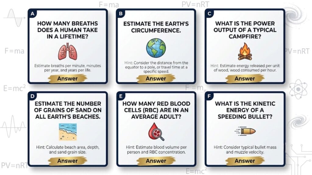
Problem A: How many molecules of air do you breathe in a single breath? (Hint: volume of one breath ~0.5 L, molar volume at STP ~22.4 L/mol) Order of magnitude answer: ~\( 10^{22} \)
Problem B: How many times does the Earth’s circumference fit across the observable universe? (Hint: observable universe diameter ~\( 10^{27} \) m, Earth’s circumference ~\( 4 \times 10^7 \) m) Order of magnitude answer: ~\( 10^{19} \)
Problem C: What is the approximate power output of a human body at rest? (Hint: food energy intake ~2000 kcal/day, 1 kcal = 4184 J) Order of magnitude answer: ~100 W (\( 10^2 \) W)
Problem D: How many grains of sand are on all of Earth’s beaches? (Hint: estimate beach area, sand depth, grain size) Order of magnitude answer: ~\( 10^{18} \) to \( 10^{19} \)
Problem E: How many red blood cells are in the human body? (Hint: blood volume ~5 L, red blood cell density ~\( 5 \times 10^6 \) cells/μL) Order of magnitude answer: ~\( 2.5 \times 10^{13} \)
Problem F: What is the kinetic energy of a flying bullet? (Hint: mass ~10 g = 0.01 kg, speed ~300 m/s) Order of magnitude answer: \( \frac{1}{2} \times 0.01 \times 300^2 = 450 \) J ~\( 10^2 \) to \( 10^3 \) J
Fermi Estimation and the Limits of Physics Knowledge
One of the deepest insights embedded in Fermi estimation is about the structure of physical knowledge itself: an enormous amount of information about the physical world can be inferred from a surprisingly small set of known facts.
The mass of the atmosphere follows from knowing atmospheric pressure and the Earth’s radius — two facts, one result. The number of cells in the body follows from knowing human size and cell size. The energy of the Sun follows from Earth’s temperature and the Stefan-Boltzmann law.
These connections — between what we know and what we can infer — are the essence of physics reasoning. Fermi estimation makes this inferential structure visible and explicit. Every time you successfully estimate an unknown from known quantities, you have demonstrated that the physical world is more interconnected than it might appear.
This is also why Fermi estimation is a diagnostic tool for physical intuition. A student who can estimate the number of atoms in a mole of gas, the range of a rifle bullet, or the temperature of the Sun’s core from first principles has demonstrated something much deeper than factual recall. They have demonstrated that they understand how physical quantities relate to each other — which is exactly what physics is about.
Conclusion
Fermi estimation is, at its core, an application of dimensional reasoning and physical intuition to problems where exact data is unavailable. The method works because the laws of physics constrain the possible answers to any physically meaningful question — and those constraints, systematically applied, produce reliable order-of-magnitude estimates from general knowledge alone.
The practice problems in this article are a starting point. The real skill comes from doing this habitually — estimating quantities you encounter in daily life, checking against actual values when possible and calibrating your intuition over time. A physicist who can look at a problem and immediately say “that’s about \( 10^{15} \) joules” or “that’s a few tens of nanometres” without calculation has internalized something that no amount of formula memorization can provide.
Practice the decomposition habit. Carry the anchor values. Trust the logarithmic statistics. And never be afraid to write something on the back of an envelope.
Learn more about What Is Dimensional Formula? Derivation, Applications & Limitations
Frequently Asked Questions
What is Fermi estimation and why is it useful?
Fermi estimation is a method of making order-of-magnitude estimates of physical quantities by decomposing an unknown into a product of individually estimable factors. It is useful because it gives reliable scale estimates without detailed data, acts as a sanity check on detailed calculations, guides experimental feasibility assessment and trains physical intuition through systematic reasoning.
How accurate are Fermi estimates?
Typically within a factor of 3–10 of the true value and almost always within one to two orders of magnitude. The method’s statistical robustness comes from the tendency of independent errors to partially cancel on a logarithmic scale. Estimates with many independent steps may drift further, but a careful five-step estimate is usually within a factor of 5 of the true answer.
What is the order of magnitude of a number?
The order of magnitude of a number is the power of 10 closest to it. For a number \( N = a \times 10^n \) with \( 1 \leq a < 10 \): if \( a < \sqrt{10} \approx 3.162 \), the order of magnitude is \( 10^n \); if \( a \geq \sqrt{10} \), it is \( 10^{n+1} \).
Why does Fermi estimation use order of magnitude rather than exact values?
Because the purpose of Fermi estimation is to determine the scale of a quantity, not its precise value. An error by a factor of 2 in each of five independent estimates compounds to an error of at most a factor of \( 2^5 = 32 \) — less than two orders of magnitude. Working in orders of magnitude keeps the arithmetic simple and focuses attention on the physics rather than the numbers.
What are the most important numbers to memorize for Fermi estimation?
The key anchor values are: Earth’s radius (\( 6.4 \times 10^6 \) m), Earth’s population (\( 8 \times 10^9 \)), speed of light (\( 3 \times 10^8 \) m/s), Avogadro’s number (\( 6 \times 10^{23} \)), atmospheric pressure (\( 10^5 \) Pa), seconds per year (\( \pi \times 10^7 \)), proton mass (\( 1.67 \times 10^{-27} \) kg) and human-scale quantities (mass ~70 kg, height ~1.7 m). With these ten anchor values, the vast majority of Fermi problems can be started.
Leave a Comment