
Introduction
Most students learn dimensional analysis as a chapter-one exercise — verify this equation, find the dimensions of that constant, convert a value from CGS to SI. It is presented as a bookkeeping tool, something to check your work before moving on to the real physics. This impression is understandable and almost entirely wrong.
Dimensional analysis is one of the most powerful reasoning techniques in applied science. Physicists, engineers and mathematicians have used it to derive results that would have taken months of detailed calculation, to design experiments that could not otherwise be afforded and to make predictions about phenomena that had never been directly observed. The technique works because the structure of physical quantities — their dimensions — carries genuine information about how nature behaves, independent of any specific theory.
This article presents seven real-world applications of dimensional analysis that go well beyond textbook exercises. Some of them will genuinely surprise you. All of them illuminate something important about why this technique is worth understanding at a deeper level than most introductory courses require.
The Core Idea: Why Dimensions Carry Information
Before the seven applications, one foundational point needs to be clear.
Physical laws are relationships between measurable quantities. Those relationships must hold regardless of the units chosen to express them — a bridge does not care whether its load is measured in kilograms or pounds. This requirement — that physical laws be independent of the choice of units — is far more constraining than it might appear. It means that any valid physical relationship must be dimensionally homogeneous: every term must carry the same dimensions.
This constraint does not just allow us to check equations. It allows us to derive them, scale them and extend them to regimes we cannot directly access. That is the power of dimensional analysis in practice.
Learn more about Dimensional Analysis Made Easy: Method, Rules and Practice Problems
Application 1: Estimating the Energy of the First Nuclear Explosion
This is perhaps the most dramatic single use of dimensional analysis in the history of science — and it became a famous story precisely because the result came from pure dimensional reasoning rather than classified calculations.
In 1950, the British physicist Geoffrey Taylor published a paper that extracted the yield of the first nuclear test explosion — the Trinity test of 1945 — from a series of declassified photographs showing the expanding fireball at different time intervals. The photographs gave the radius of the fireball as a function of time. Everything else came from dimensional analysis.
The Setup
Taylor assumed that the blast wave radius \( R \) at time \( t \) after detonation depended on:
- The energy released \( E \) (the quantity to be found)
- The density of the surrounding air \( \rho \)
- Time \( t \)
He wrote:
\[ R = k \cdot E^a \cdot \rho^b \cdot t^c \]
Where \( k \) is a dimensionless constant of order 1.
Dimensional Analysis
Taking dimensions:
\[ [R] = L, \quad [E] = ML^2T^{-2}, \quad [\rho] = ML^{-3}, \quad [t] = T \]
\[ L = (ML^2T^{-2})^a \cdot (ML^{-3})^b \cdot T^c \]
\[ L^1 M^0 T^0 = M^{a+b} L^{2a-3b} T^{-2a+c} \]
Comparing exponents:
- M: \( a + b = 0 \Rightarrow b = -a \)
- T: \( -2a + c = 0 \Rightarrow c = 2a \)
- L: \( 2a – 3b = 1 \Rightarrow 2a + 3a = 1 \Rightarrow a = \frac{1}{5} \)
Therefore:
\[ b = -\frac{1}{5}, \quad c = \frac{2}{5} \]
\[ R = k \left(\frac{E t^2}{\rho}\right)^{1/5} \]
Extracting the Energy
Rearranging:
\[ E = k^5 \cdot \frac{\rho R^5}{t^2} \]
Taylor read values of \( R \) and \( t \) from the published photographs, used the known density of air \( \rho \approx 1.2 \text{ kg/m}^3 \), set \( k \approx 1 \) (confirmed by more detailed calculation) and obtained:
\[ E \approx 10^{14} \text{ J} \approx 20 \text{ kilotons of TNT} \]
The actual yield was approximately 21 kilotons. Taylor’s estimate, from photographs and dimensional analysis alone, was accurate to within 5%.
The result caused considerable concern among US officials, since it demonstrated that a skilled physicist could extract classified nuclear test yields from publicly available photographs using nothing but physics reasoning.
What This Shows
Dimensional analysis does not just verify known results. With the right physical insight about which variables matter, it can extract quantitative information from qualitative observations with remarkable precision.
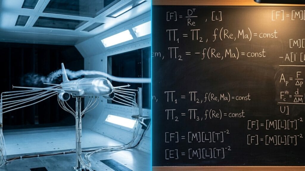
Application 2: Wind Tunnel Testing and the Reynolds Number
When an engineer designs a new aircraft, testing a full-scale prototype in a wind tunnel is often impossible — the tunnel may not be large enough, the cost may be prohibitive, or the speeds involved may be unachievable at full scale. Instead, scale models are tested.
But here is the problem: a scale model at the same airspeed as the full aircraft will not experience the same aerodynamic forces in proportion to its size. The physics of fluid flow depends not just on speed and size, but on their combination with the fluid’s properties. Unless the model test reproduces the right dimensionless combination of these quantities, the results do not scale.
The relevant dimensionless combination is the Reynolds number:
\[ Re = \frac{\rho v L}{\mu} \]
Where:
- \( \rho \) = fluid density \( [ML^{-3}] \)
- \( v \) = flow velocity \( [LT^{-1}] \)
- \( L \) = characteristic length (e.g., wing chord length) \( [L] \)
- \( \mu \) = dynamic viscosity \( [ML^{-1}T^{-1}] \)
Dimensional check:
\[ [Re] = \frac{ML^{-3} \cdot LT^{-1} \cdot L}{ML^{-1}T^{-1}} = \frac{ML^{-1}T^{-1}}{ML^{-1}T^{-1}} = M^0L^0T^0 \]
The Reynolds number is dimensionless — as it must be, since it is a ratio of inertial to viscous forces, two quantities that cancel in dimensions.
The Scaling Principle
For a model test to correctly predict full-scale behavior, the Reynolds number of the model test must equal the Reynolds number of the full-scale flow. This is the principle of dynamic similarity.
If the model is scaled down by a factor of 10 (L is 10 times smaller), the test fluid’s velocity must be increased by a factor of 10 (or a denser fluid must be used) to maintain the same Re. This is precisely what wind tunnels do — they adjust airspeed, air pressure, or use substitute fluids to achieve dynamic similarity with the full-scale aircraft at realistic flight conditions.
Why This Matters
The Reynolds number was derived by dimensional analysis of the Navier-Stokes equations by Osborne Reynolds in the 1880s. It remains the central organizing concept of fluid mechanics. Every fluid dynamics problem — from blood flow in arteries to airflow over a Mars lander — is analyzed in terms of the Reynolds number and other dimensionless groups derived by the same technique.
This application is not a classroom curiosity. It is the practical foundation of every aerodynamic and hydrodynamic test ever conducted on a model.

Application 3: The Buckingham Pi Theorem — Turning Complex Problems into Manageable Ones
Individual dimensional analysis of simple systems is impressive. The formal generalization of the technique — the Buckingham Pi theorem — is transformative.
The Theorem
If a physical system is described by \( n \) variables involving \( k \) independent fundamental dimensions, then the relationship between those variables can be expressed as a function of \( n – k \) independent dimensionless groups (called Pi groups, denoted \( \Pi_1, \Pi_2, \ldots \)).
\[ f(q_1, q_2, \ldots, q_n) = 0 \quad \Longleftrightarrow \quad F(\Pi_1, \Pi2, \ldots, \Pi{n-k}) = 0 \]
Why This Is Powerful
Suppose you are studying a problem involving 8 physical variables and 3 fundamental dimensions (M, L, T). Full experimentation — mapping out the relationship between 8 variables — would require an astronomical number of experiments. The Buckingham Pi theorem reduces this to a relationship between \( 8 – 3 = 5 \) dimensionless groups. The number of independent experiments required drops from practically infinite to tractable.
A Concrete Example: Drag on a Sphere
The drag force \( F_D \) on a sphere moving through a viscous fluid depends on:
| Variable | Symbol | Dimensions |
| Drag force | \( F_D \) | \( MLT^{-2} \) |
| Fluid density | \( \rho \) | \( ML^{-3} \) |
| Fluid velocity | \( v \) | \( LT^{-1} \) |
| Sphere diameter | \( D \) | \( L \) |
| Fluid viscosity | \( \mu \) | \( ML^{-1}T^{-1} \) |
5 variables, 3 dimensions → \( 5 – 3 = 2 \) dimensionless groups.
The two groups turn out to be:
\[ \Pi_1 = \frac{F_D}{\rho v^2 D^2} \quad \text{(drag coefficient } C_D\text{)} \]
\[ \Pi_2 = \frac{\rho v D}{\mu} \quad \text{(Reynolds number } Re\text{)} \]
The full relationship \( F_D = f(\rho, v, D, \mu) \) reduces to:
\[ C_D = g(Re) \]
A function of four variables becomes a function of one variable. Experimentally mapping this single relationship requires far fewer measurements than exploring the original four-variable space.
This is how Stokes’ law (\( F_D = 3\pi\mu v D \) for low Re) and the general drag formula are both special cases of the same dimensionless relationship.
Application 4: Predicting the Orbital Period of Planets — Kepler’s Third Law from Dimensions
Johannes Kepler discovered his third law empirically in 1619: the square of a planet’s orbital period is proportional to the cube of its semi-major axis. Dimensional analysis can derive this relationship without any knowledge of Newtonian mechanics.
The Setup
Assume the orbital period \( T \) of a planet depends on:
- The semi-major axis \( r \) (characteristic orbital distance) \( [L] \)
- The mass of the Sun \( M \) \( [M] \)
- The gravitational constant \( G \) \( [M^{-1}L^3T^{-2}] \)
Write:
\[ T = k \cdot r^a \cdot M^b \cdot G^c \]
Dimensional Analysis
\[ [T] = L^a \cdot M^b \cdot (M^{-1}L^3T^{-2})^c = M^{b-c} L^{a+3c} T^{-2c} \]
Comparing exponents:
- T: \( -2c = 1 \Rightarrow c = -\frac{1}{2} \)
- M: \( b – c = 0 \Rightarrow b = -\frac{1}{2} \)
- L: \( a + 3c = 0 \Rightarrow a = \frac{3}{2} \)
\[ T = k \cdot r^{3/2} \cdot M^{-1/2} \cdot G^{-1/2} = k\sqrt{\frac{r^3}{GM}} \]
This is Kepler’s Third Law. The full result from Newtonian mechanics is \( T = 2\pi\sqrt{r^3/GM} \) — dimensional analysis gives the correct form and the constant \( k = 2\pi \) requires the full theoretical treatment to recover.
What This Shows
Dimensional analysis can reproduce Kepler’s empirical law purely from a reasonable guess about which variables matter. No force laws, no calculus, no integration of orbits — just dimensions. This is the technique at its most elegant.
Application 5: Medical Physics — Drug Dosage Scaling Across Species
The application of dimensional analysis to pharmacology and medical research is less famous than its use in fluid mechanics but equally important in practice. When a drug is tested in mice and then approved for human use, the dosage must be scaled appropriately. Getting this wrong — even by a factor of two — can be the difference between therapeutic and toxic.
The Problem
Drug metabolism in mammals depends on body mass and metabolic rate. Metabolic rate scales non-linearly with body mass — a relationship known as Kleiber’s law:
\[ P \propto M^{3/4} \]
Where \( P \) is metabolic rate and \( M \) is body mass. This \( 3/4 \) exponent has been empirically confirmed across species ranging from mice to elephants and dimensional analysis — combined with fractal geometry arguments about the structure of biological distribution networks — provides a theoretical basis for why this exponent is \( 3/4 \) and not \( 1 \) or \( 2/3 \).
Dimensional Scaling of Drug Dose
For a drug cleared by metabolic processes, the dose per kilogram body mass that produces the same therapeutic effect scales as:
\[ \text{Dose (per kg)} \propto M^{-1/4} \]
This means a mouse (body mass ~ 25 g) requires a dose per kilogram that is approximately:
\[ \left(\frac{25 \times 10^{-3}}{70}\right)^{-1/4} \approx 7 \text{ times higher per kg} \]
than a human (body mass ~ 70 kg).
A pharmacologist who simply scaled the mouse dose linearly to human body weight would overshoot the human dose by a factor of approximately 7 — with potentially fatal consequences.
The FDA and regulatory agencies around the world use scaling relationships derived from dimensional and allometric analysis as a standard first step in translating animal study results to human dose recommendations. Dimensional reasoning is not just academic here — it directly affects patient safety.

Application 6: Structural Engineering — Why Giants Cannot Exist
This application of dimensional analysis touches a question that has fascinated biologists and engineers for centuries: why do animals have the body proportions they do and is there a physical limit to how large a land animal can be?
Galileo’s Insight
Galileo Galilei was the first to analyze this problem systematically, in his 1638 Dialogue Concerning Two New Sciences. He argued that bones must support the weight of the animal and that weight scales with volume (and hence with the cube of linear size), while bone cross-sectional area scales with the square of linear size.
The Dimensional Argument
Consider a geometrically similar animal scaled up by a factor \( \lambda \) in all linear dimensions:
- Linear dimensions: \( \times \lambda \)
- Body volume (and mass): \( \times \lambda^3 \)
- Weight \( W \propto m \): \( \times \lambda^3 \)
- Bone cross-sectional area \( A \propto L^2 \): \( \times \lambda^2 \)
- Stress on bone \( \sigma = W/A \): \( \times \lambda^3/\lambda^2 = \times \lambda \)
This is the key result: bone stress increases linearly with size. If you double all dimensions of an animal, bone stress doubles. If you scale up by a factor of ten, bone stress increases tenfold.
Since bone has a fixed ultimate compressive strength (approximately 170 MPa for cortical bone), there is a maximum size at which a geometrically similar animal’s bones would fail under its own weight. Beyond that size, the animal must either:
- Change its geometry — making bones proportionally thicker relative to body length (which is exactly what elephant bones look like compared to mouse bones)
- Change its mode of locomotion — very large animals move more slowly and spend more time with multiple limbs on the ground
- Use a medium that partially supports its weight — which is why the largest animals in Earth’s history (blue whale, some sauropod dinosaurs) are or were aquatic or semi-aquatic
This dimensional scaling argument — mass scales as \( L^3 \), strength-limited area as \( L^2 \) — explains why you will never see a land animal the size of a blue whale and why giant insects from science fiction are physically impossible (their respiratory and skeletal systems cannot scale the way the stories require).
Application 7: Cosmology and Planck Units — The Natural Scale of the Universe
The most philosophically profound application of dimensional analysis is the construction of the Planck unit system — a set of natural units derived entirely from dimensional analysis of the fundamental constants of nature.
The Observation
Three fundamental constants of physics have the following dimensions:
| Constant | Symbol | Value (SI) | Dimensions |
| Speed of light | \( c \) | \( 3 \times 10^8 \text{ m/s} \) | \( LT^{-1} \) |
| Planck’s constant | \( \hbar = h/2\pi \) | \( 1.055 \times 10^{-34} \text{ J·s} \) | \( ML^2T^{-1} \) |
| Gravitational constant | \( G \) | \( 6.674 \times 10^{-11} \text{ N·m}^2/\text{kg}^2 \) | \( M^{-1}L^3T^{-2} \) |
These three constants — and only these three — can be combined to form unique quantities with the dimensions of length, time and mass. The combination is determined entirely by dimensional analysis:
Planck Length
\[ \ell_P = \sqrt{\frac{\hbar G}{c^3}} \]
Dimensional check:
\[ \left[\frac{\hbar G}{c^3}\right] = \frac{ML^2T^{-1} \cdot M^{-1}L^3T^{-2}}{(LT^{-1})^3} = \frac{L^5T^{-3}}{L^3T^{-3}} = L^2 \]
\[ \ell_P = \sqrt{L^2} = L \quad \checkmark \]
\[ \ell_P \approx 1.616 \times 10^{-35} \text{ m} \]
Planck Time
\[ t_P = \sqrt{\frac{\hbar G}{c^5}} \approx 5.391 \times 10^{-44} \text{ s} \]
Planck Mass
\[ m_P = \sqrt{\frac{\hbar c}{G}} \approx 2.176 \times 10^{-8} \text{ kg} \]
What the Planck Scale Means
The Planck units are not merely convenient. They represent the scale at which both quantum mechanics and general relativity simultaneously become important — the scale where the current frameworks of physics break down and a theory of quantum gravity is needed.
The Planck length is the smallest length scale at which the concept of space itself, as described by general relativity, remains meaningful. Below this scale, quantum fluctuations in the geometry of spacetime become comparable to the geometry itself.
The entire Planck unit system — length, time, mass, temperature and charge — is constructed purely by dimensional analysis of fundamental constants. No experiment, no arbitrary choice of unit, no human convention. The Planck scale is where the universe sets its own yardstick.
Learn more about Planck Units: The Natural Unit System That Defined the Universe’s Scale
Why These Applications All Work: The Deeper Structure
All seven applications share a common foundation: they exploit the fact that physical laws must be expressible in dimensionless form. This is not an assumption — it is a theorem, formally stated as the Buckingham Pi theorem, that follows from the requirement that physical laws be independent of the choice of units.
When Geoffrey Taylor read photographs of a nuclear explosion and used dimensional analysis to extract the energy yield, he was using this principle. When an aeronautical engineer sets the wind tunnel speed to achieve the right Reynolds number, they are using this principle. When Max Planck combined \( c \), \( \hbar \) and \( G \) to construct a natural unit system, he was using this principle.
The same tool — dimensional analysis — works across all these domains because the underlying mathematical structure is the same in all of them. The dimensions of physical quantities carry information about the structure of natural law. Exploiting that information is what the technique does.
Learn more about Fermi Estimation in Physics: Using Order of Magnitude to Solve Real Problems

Summary: Seven Applications at a Glance
| Application | Domain | What Dimensional Analysis Did |
| 1. Nuclear yield from photographs | Nuclear physics / History | Extracted a classified energy value from public photographs |
| 2. Wind tunnel scaling (Reynolds number) | Aerodynamics / Engineering | Enabled model testing to predict full-scale aerodynamic behaviour |
| 3. Buckingham Pi theorem | All of physics and engineering | Reduced multi-variable problems to manageable dimensionless groups |
| 4. Kepler’s Third Law | Orbital mechanics / Astronomy | Derived the T² ∝ r³ relationship without Newton’s laws |
| 5. Drug dosage across species | Medical physics / Pharmacology | Correctly scaled drug doses between test animals and humans |
| 6. Limits of biological size | Biophysics / Structural engineering | Explained why land giants cannot exist through geometric scaling |
| 7. Planck units | Cosmology / Quantum gravity | Constructed the natural scale of the universe from fundamental constants |
Conclusion
Dimensional analysis, taught as a first-week verification tool, turns out to be a first-rate instrument of scientific discovery. Geoffrey Taylor used it to embarrass national security. Reynolds used it to make aerodynamic modeling possible. Buckingham turned it into a systematic framework for reducing experimental complexity. Galileo used it to understand why biology has the shapes it does. And Planck used it to find the natural scale built into the laws of physics themselves.
The technique works for one reason: nature does not care what units you use. Any true physical relationship must be expressible without reference to any particular unit system — which means it must be expressible in terms of dimensionless groups. Dimensional analysis finds those groups. And in the structure of those groups lies genuine knowledge about how the physical world works.
When you next sit down with a dimensional analysis problem — checking an equation, finding the dimensions of a constant, converting between systems — it is worth remembering that you are using the same technique that revealed the yield of a nuclear bomb, enabled every aircraft ever wind-tunnel tested and defined the fundamental scale of the universe.
Learn more about Dimensional Analysis Made Easy: Method, Rules and Practice Problems
Frequently Asked Questions
What is the most famous real-world application of dimensional analysis?
Geoffrey Taylor’s 1950 extraction of the Trinity nuclear test yield from declassified photographs is arguably the most famous single application. Using dimensional analysis of the expanding blast radius, Taylor deduced the explosive yield as approximately 20 kilotons of TNT — accurate to within 5% of the classified true value, from photographs alone.
What is the Buckingham Pi theorem and why is it important?
The Buckingham Pi theorem states that any physical relationship between \( n \) variables involving \( k \) independent dimensions can be expressed as a relationship between \( n – k \) dimensionless groups. It is important because it systematically reduces the complexity of experimental and theoretical problems — a relationship that seemed to require testing eight variables might reduce to a function of just five dimensionless groups, dramatically cutting the required experimental work.
How is dimensional analysis used in aeronautical engineering?
Aeronautical engineers use dimensional analysis to identify the Reynolds number and other dimensionless parameters that govern fluid flow. When testing a scale model in a wind tunnel, the engineers adjust airspeed or fluid density to match the Reynolds number of the full-scale aircraft at its operating conditions. This ensures that the model test results scale correctly to full-size predictions — a process called dynamic similarity.
Can dimensional analysis be used in biology?
Yes. Dimensional analysis and allometric scaling — the study of how biological properties scale with body size — are closely related. Kleiber’s law (metabolic rate scales as \( M^{3/4} \)) and the scaling of drug dosages across species both use dimensional and geometric scaling arguments. The structural limits on animal size (why giants cannot exist on land) are a direct application of the \( L^3 \) versus \( L^2 \) scaling of weight versus bone strength.
What are Planck units and how are they derived?
Planck units are a system of natural units derived by dimensional analysis of the three fundamental constants \( c \), \( \hbar \) and \( G \). These three constants uniquely determine units of length (\( \ell_P \approx 1.6 \times 10^{-35} \) m), time (\( t_P \approx 5.4 \times 10^{-44} \) s) and mass (\( m_P \approx 2.2 \times 10^{-8} \) kg) purely through dimensional combination. No experiment or human convention is involved — the Planck scale is built into the structure of the fundamental constants.
Why does dimensional analysis work even without knowing the underlying physics?
Because dimensional analysis exploits a mathematical property of physical laws — their independence from the choice of units — without requiring knowledge of the specific form of those laws. As long as you correctly identify the relevant variables, the dimensions alone constrain the possible form of the relationship. The undetermined dimensionless constant (like \( 2\pi \) in Kepler’s law) requires the full physics to determine, but the dimensional structure of the result does not.
How does dimensional analysis relate to the scaling of biological organisms?
As a biological organism scales up in size, its mass grows as \( L^3 \) while cross-sectional areas grow as \( L^2 \). The stress on load-bearing structures therefore grows as \( L \). This means larger animals need proportionally stronger (thicker) bones and move differently. Beyond a certain size, no geometrically similar land animal can support its own weight — which is why the largest animals that ever lived on land had very different body proportions from smaller relatives and why the very largest animals exist in water.
Leave a Comment