

Introduction
There is a statement that every physics student eventually encounters, usually in the first week of a practical course: no measurement is exact. Stated that bluntly, it sounds like a limitation — an admission that physics cannot quite get things right. The reality is almost the opposite. Understanding why uncertainty always exists and how to quantify it honestly, is what gives a measurement its scientific meaning. A result without an uncertainty estimate is not a humble admission of imprecision. It is an overclaim — an assertion of exactness that no physical measurement can support.
This article explains what measurement uncertainty is, why it is unavoidable, how it originates from physical principles rather than just experimental carelessness, how it is quantified and what it means to report a result correctly. These ideas appear at the beginning of every physics education, but they run much deeper than most introductory courses reveal.
What Is Measurement Uncertainty?
Measurement uncertainty is the quantitative characterization of the range of values within which the true value of a measured quantity can reasonably be expected to lie.
When you write a measurement as:
\[ x = \bar{x} \pm u \]
you are saying that the true value of the quantity being measured lies in the interval \( [\bar{x} – u,\ \bar{x} + u] \) with a specified level of confidence. The \( \pm u \) is not an apology. It is a claim about the reliability of the measurement — a quantitative statement about how much the reported value can be trusted.
There are several important distinctions to establish at the outset.
Uncertainty is not the same as error. Error, in the strict sense, is the difference between the measured value and the true value: \( e = x\text{measured} – x\text{true} \). Error requires knowing the true value. Uncertainty is an estimate of the likely magnitude of the error, made without necessarily knowing the true value. Uncertainty is what you report; error is what you would compute if you had a perfect standard.
Uncertainty is not the same as mistake. A mistake (gross error) is a blunder — misreading a scale, recording the wrong digit, using the wrong formula. Mistakes can be eliminated by care. Uncertainty cannot be eliminated, only reduced and quantified.
Uncertainty is not the same as precision. Precision describes how well measurements agree with each other (reproducibility). Uncertainty describes the range of possible values for the true result. A set of highly reproducible measurements can still have high uncertainty if there is a systematic bias.
Why Measurement Uncertainty Always Exists
The permanence of measurement uncertainty is not a technological limitation that will eventually be overcome with better instruments. It has physical roots that go much deeper than instrument quality.
Reason 1: The Finite Resolution of Every Measuring Instrument
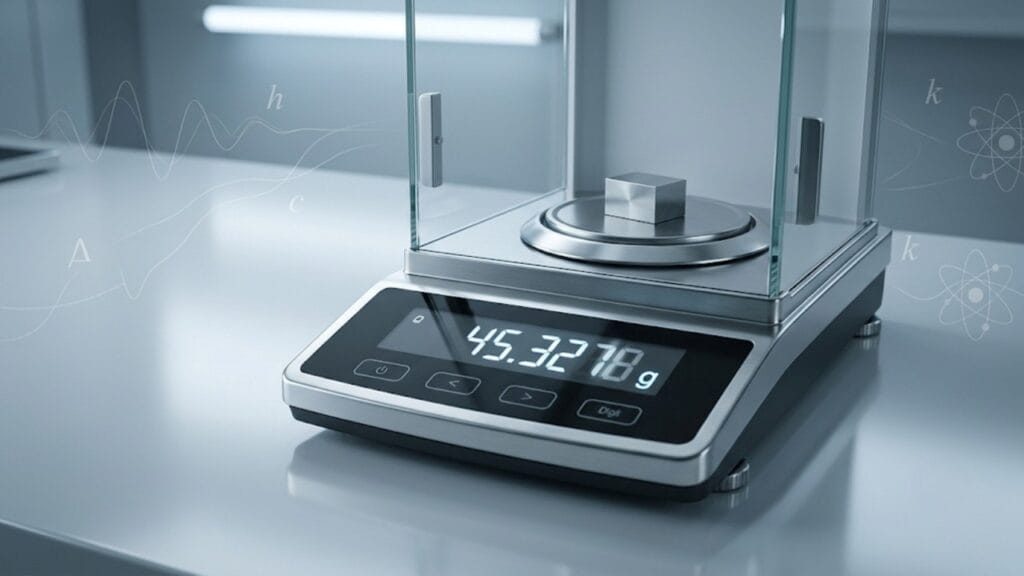
Every measuring instrument has a least count — the smallest increment it can distinguish. A ruler graduated in millimetres cannot distinguish lengths differing by less than half a millimetre, no matter how carefully it is read. A digital balance displaying three decimal places in grams cannot distinguish masses differing by less than half a milligram.
This resolution limit is a physical property of the instrument, not a flaw. No instrument can have zero least count without infinite resolution, which would require infinite precision in the physical mechanism of the measurement.
The contribution of resolution to uncertainty is approximately:
\[ u_\text{resolution} = \pm \frac{\text{Least Count}}{2} \]
or, by the conservative school-level convention:
\[ u_\text{resolution} = \pm \text{Least Count} \]
This is the irreducible floor — the minimum possible uncertainty from reading the instrument, even with perfect technique.
Reason 2: Environmental Fluctuations
Every measurement is made in an environment that is never perfectly controlled. Temperature fluctuates. Air currents disturb sensitive balances. Electrical noise enters signals. Vibrations propagate through building structures. The object being measured may be changing during the measurement process — warming up, cooling down, flexing under load, expanding or contracting.
These environmental fluctuations produce random variations in readings. They cannot be eliminated — they can only be reduced by better environmental control and quantified by statistical analysis of repeated readings.
Reason 3: Observer Effects
In classical physics, reading an instrument involves judgment. When a pointer falls between two scale divisions, the observer estimates its position. Different observers will estimate differently; the same observer will estimate slightly differently on repeated readings. The reaction time in starting and stopping a stopwatch varies. The angle at which an observer views a scale introduces parallax error of variable magnitude.
These observer effects are irreducibly random for any human-based measurement. Automated instruments reduce but do not eliminate this — electronic noise, quantization error and threshold effects introduce their own random contributions.
Reason 4: The Heisenberg Uncertainty Principle
At the deepest level, measurement uncertainty has a quantum mechanical origin that transcends all instrument limitations and environmental control.
The Heisenberg Uncertainty Principle states:
\[ \Delta x \cdot \Delta p \geq \frac{\hbar}{2} \]
Where \( \Delta x \) is the uncertainty in position and \( \Delta p \) is the uncertainty in momentum and \( \hbar = h/2\pi \) is the reduced Planck constant.
Similarly:
\[ \Delta E \cdot \Delta t \geq \frac{\hbar}{2} \]
These are not statements about instrument limitations. They are fundamental statements about physical reality — position and momentum, or energy and time, cannot simultaneously have definite values at the quantum level. This is not a consequence of disturbing a system by measuring it (though that does occur). It is a property of quantum states themselves: a state with definite position is genuinely a superposition of many momenta and vice versa.
For macroscopic measurements, quantum uncertainty is utterly negligible — the Planck constant \( \hbar \approx 10^{-34} \) J·s is so small that the uncertainty it implies for macroscopic masses and velocities is far below anything a physical instrument can resolve. But for atomic and subatomic measurements, quantum uncertainty is the dominant source of irreducible uncertainty.
More fundamentally, the Heisenberg principle shows that uncertainty is not accidental — it is woven into the fabric of physical law. Even a perfect instrument operated in a perfect environment by a perfect observer would face quantum uncertainty at sufficiently small scales.
Types of Uncertainty: A Systematic Classification
Measurement uncertainty in physics is classified into two types, designated Type A and Type B by the international standard (ISO Guide to the Expression of Uncertainty in Measurement, known as the GUM).
Type A Uncertainty: Statistical Evaluation
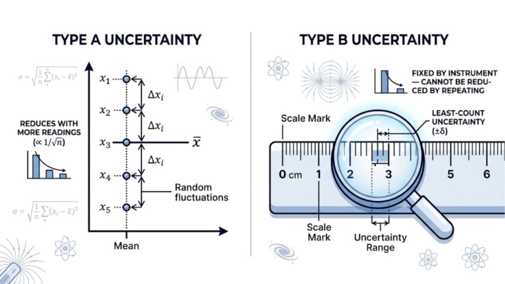
Type A uncertainty is evaluated by statistical analysis of a series of repeated measurements. It is what most school-level physics courses call “random error.”
The mean of \( n \) repeated measurements:
\[ \bar{x} = \frac{1}{n}\sum_{i=1}^{n} x_i \]
The mean absolute error (used in school-level physics):
\[ \overline{\Delta x} = \frac{1}{n}\sum_{i=1}^{n} |x_i – \bar{x}| \]
The standard deviation of the measurements (used in more advanced treatment):
\[ s = \sqrt{\frac{1}{n-1}\sum_{i=1}^{n}(x_i – \bar{x})^2} \]
The standard uncertainty of the mean (standard error of the mean):
\[ u_A = \frac{s}{\sqrt{n}} \]
Type A uncertainty decreases as more measurements are taken, scaling approximately as \( 1/\sqrt{n} \). This is why repeating a measurement improves precision — but with diminishing returns. Quadrupling the number of readings halves the Type A uncertainty.
Type B Uncertainty: Non-Statistical Evaluation
Type B uncertainty is evaluated by means other than statistical analysis. It includes:
- Instrument resolution: \( u = \frac{1}{2} \times \text{LC} \) (or \( \pm \text{LC} \) by the conservative approach)
- Calibration uncertainty: Stated in the instrument’s calibration certificate or datasheet
- Manufacturer specifications: Maximum error stated in the instrument manual
- Environmental effects: Temperature coefficients, humidity sensitivity, known electromagnetic interference
- Rounding of tabulated values: When using a value from a table or formula that has been rounded
Type B uncertainty does not decrease with more measurements. It is fixed by the instrument and the method. It can only be reduced by using a better-calibrated instrument, controlling environmental conditions, or applying corrections.
Combined Uncertainty
When multiple independent sources of uncertainty contribute, the combined uncertainty is found by adding them in quadrature (for independent sources):
\[ u_\text{combined} = \sqrt{u_1^2 + u_2^2 + u_3^2 + \cdots} \]
At school level, a simpler worst-case approach adds them linearly:
\[ u_\text{combined} = u_1 + u_2 + u_3 + \cdots \]
The quadrature addition is statistically correct for independent sources; the linear addition is more conservative and is standard practice in CBSE and competitive exam error analysis.
How to Express and Report Uncertainty
The correct reporting format for a measurement with uncertainty is:
\[ x = \bar{x} \pm u \text{ (unit)} \]
Example: \( L = 12.35 \pm 0.05 \text{ cm} \)
This means: the true length is most likely between 12.30 cm and 12.40 cm.
Rules for Reporting
Rule 1: The uncertainty should be rounded to one or two significant figures. Reporting \( u = 0.0473 \) cm is excessive — it implies you know the uncertainty itself to four significant figures, which is rarely justified. Round to \( u = 0.05 \) cm.
Rule 2: The result value should be rounded to match the decimal place of the uncertainty. If \( u = 0.05 \) cm, the result should be reported to the nearest 0.05 or 0.01 cm — not to seven decimal places.
Rule 3: The unit must be stated explicitly. \( 12.35 \pm 0.05 \) is incomplete; \( 12.35 \pm 0.05 \text{ cm} \) is complete.
Rule 4: Uncertainty is always positive. Writing \( u = -0.05 \) cm is physically meaningless.
Relative and Percentage Uncertainty
Relative uncertainty:
\[ u_r = \frac{u}{\bar{x}} \]
Percentage uncertainty:
\[ u_\% = \frac{u}{\bar{x}} \times 100\% \]
These are the dimensionless forms used in error propagation and in comparative assessment of measurement quality.
Uncertainty vs Error: A Critical Distinction for Exams
The terms uncertainty and error are often used interchangeably in Indian school physics, but they carry technically distinct meanings that examiners increasingly recognize:
| Concept | Meaning | Requires True Value? | Can Be Eliminated? |
| Error | \( x\text{measured} – x\text{true} \) | Yes | No (but can be corrected for systematic) |
| Uncertainty | Estimated range of possible errors | No | No |
| Mistake (Gross error) | Blunder in reading or recording | No | Yes, by care |
| Accuracy | Closeness to true value | Yes (comparison) | Systematic errors can be corrected |
| Precision | Reproducibility of readings | No | Random errors can be reduced |
In practice, at the school level:
- “Absolute error” ≈ absolute uncertainty (\( \overline{\Delta x} \))
- “Relative error” ≈ relative uncertainty (\( u/\bar{x} \))
- “Percentage error” ≈ percentage uncertainty (\( u/\bar{x} \times 100\% \))
The school-level formulas treat these concepts as equivalent, which is a reasonable simplification. Understanding the underlying distinction helps when questions use non-standard terminology.
Learn more about Absolute Error, Relative Error and Percentage Error: A Complete Guide
Uncertainty Propagation: When You Calculate From Measurements
Every time a derived quantity is calculated from measured values, uncertainties in the measurements propagate into the result. The propagation rules are:
For sums and differences \( Z = A \pm B \):
\[ \Delta Z = \Delta A + \Delta B \]
For products and quotients \( Z = AB \) or \( Z = A/B \):
\[ \frac{\Delta Z}{Z} = \frac{\Delta A}{A} + \frac{\Delta B}{B} \]
For powers \( Z = A^n \):
\[ \frac{\Delta Z}{Z} = |n| \cdot \frac{\Delta A}{A} \]
General formula \( Z = A^p B^q / C^r \):
\[ \frac{\Delta Z}{Z} = p\frac{\Delta A}{A} + q\frac{\Delta B}{B} + r\frac{\Delta C}{C} \]
These rules represent the worst-case (maximum) propagation — the assumption that all individual uncertainties act in the same direction simultaneously. For independent random uncertainties, the quadrature formula gives a more realistic (smaller) combined uncertainty:
\[ \left(\frac{\Delta Z}{Z}\right)^2 = \left(p\frac{\Delta A}{A}\right)^2 + \left(q\frac{\Delta B}{B}\right)^2 + \left(r\frac{\Delta C}{C}\right)^2 \]
At school level, the linear (worst-case) formula is always used. The quadrature formula appears in undergraduate and research contexts.
Learn more about Propagation of Errors in Physics Calculations: Rules, Formulas & Examples
The Measurement Model: What a Reported Value Actually Claims
When a physicist reports a measurement as \( x = \bar{x} \pm u \), they are making a specific claim about the relationship between their reported value and the true value. The nature of that claim depends on the confidence level specified.
68% Confidence Interval
For a measurement process with Gaussian (normal) random errors, the standard uncertainty \( u = s/\sqrt{n} \) defines a 68% confidence interval — meaning there is approximately a 68% probability that the true value lies within \( [\bar{x} – u, \bar{x} + u] \).
95% Confidence Interval
The expanded uncertainty \( U = 2u \) defines a 95% confidence interval — approximately a 95% probability that the true value lies within \( [\bar{x} – 2u, \bar{x} + 2u] \).
99.7% Confidence Interval
The \( 3u \) interval covers approximately 99.7% — the three-sigma rule.
At school level, uncertainty is typically reported without specifying a confidence level and the interval is interpreted as a reasonable range for the true value. This is adequate for the purpose of checking consistency and learning experimental reasoning.
Compatibility of Results: When Do Two Measurements Agree?
One of the most practically important uses of uncertainty is determining whether two measurements of the same quantity are consistent — whether they could both be measuring the same true value within their stated uncertainties.
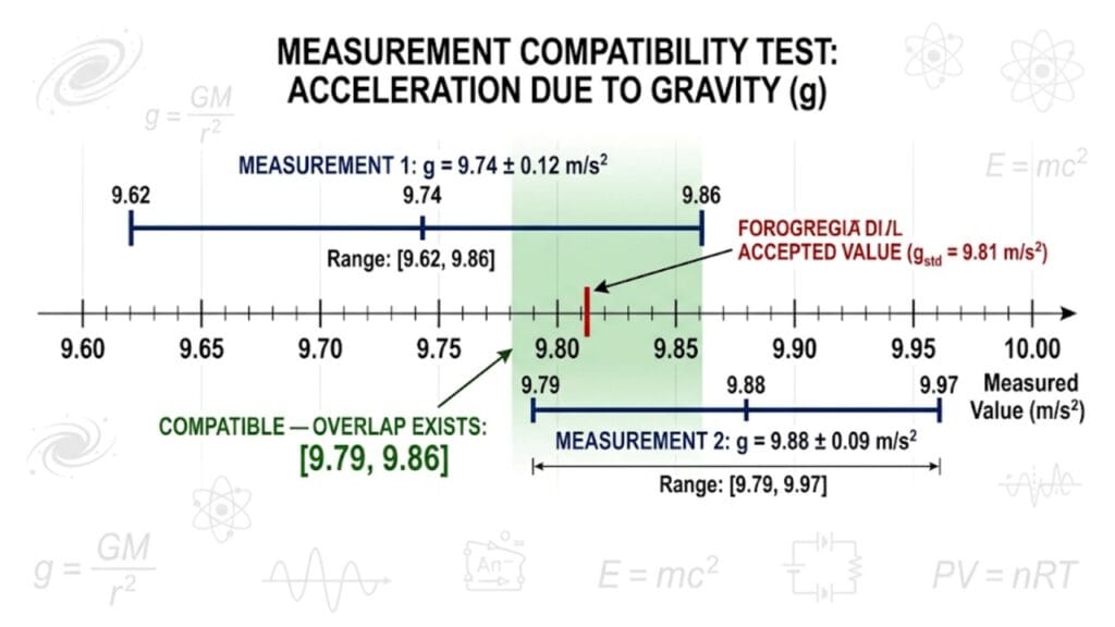
Two measurements \( x_1 = \bar{x}_1 \pm u_1 \) and \( x_2 = \bar{x}_2 \pm u_2 \) are considered compatible if their uncertainty intervals overlap:
\[ |\bar{x}_1 – \bar{x}_2| \leq u_1 + u_2 \]
Example: Student A measures \( g = 9.74 \pm 0.12 \) m/s² and student B measures \( g = 9.88 \pm 0.09 \) m/s². Are these consistent?
\[ |9.74 – 9.88| = 0.14 \] \[ u_1 + u_2 = 0.12 + 0.09 = 0.21 \]
Since \( 0.14 \leq 0.21 \), the measurements are compatible — the discrepancy is within the combined uncertainty. Both could plausibly be measuring the same true value of \( g \).
If \( |\bar{x}_1 – \bar{x}_2| > u_1 + u_2 \), the results are incompatible — the discrepancy is larger than can be accounted for by the stated uncertainties, suggesting either a systematic error in one measurement, an underestimated uncertainty, or a genuine physical difference.
This compatibility test is one of the most important outcomes of reporting uncertainty correctly. Without uncertainty estimates, two measurements with different numerical values cannot be compared meaningfully — you cannot know whether the difference is significant or not.
Why Physicists Distinguish Random and Systematic Uncertainty Separately
A result with both random and systematic uncertainties is often reported as:
\[ x = \bar{x} \pm u\text{random} \text{ (stat)} \pm u\text{systematic} \text{ (syst)} \]
The reason for keeping them separate is diagnostic. Consider a measurement that gives:
\[ g = 9.62 \pm 0.03 \text{ (stat)} \pm 0.15 \text{ (syst)} \text{ m/s}^2 \]
The statistical uncertainty is small — the measurement is highly reproducible. But the systematic uncertainty is large — something in the method or instrument is biased. The combined result is not very accurate despite being very precise.
The path to improvement is clear: investigating and correcting the systematic bias would reduce \( u\text{syst} \) from 0.15 to something smaller. Taking more readings would only reduce \( u\text{stat} \), which is already small — it would accomplish nothing useful.
If only a combined uncertainty were reported, this diagnostic distinction would be lost and the experimenter might waste effort on the wrong improvement.
Learn more about Top 5 Errors in Physics Measurements and How to Minimize Them
Uncertainty in the Context of Significant Figures
Significant figures are the practical encoding of uncertainty in a reported number. The number of significant figures in a measurement communicates the approximate scale of its uncertainty.
A measurement reported as \( 4.53 \) cm implies uncertainty in the last digit — an uncertainty of roughly \( \pm 0.01 \) cm. A measurement reported as \( 4.5 \) cm implies uncertainty in the tenths digit — roughly \( \pm 0.1 \) cm.
The rules governing significant figures in calculations (fewest significant figures for multiplication; fewest decimal places for addition) are approximations to the full uncertainty propagation analysis. They give the correct order-of-magnitude treatment of how precision flows through calculations without requiring explicit uncertainty estimates at every step.
This is why both topics — significant figures and uncertainty — are taught together in Units and Measurements. They are two levels of treatment of the same underlying question: how reliable is a computed number, given the reliability of the measurements that went into it?
Learn more about How to Find Significant Figures: Rules, Examples & Common Mistakes
The International Standard: The GUM
The authoritative international standard for expressing measurement uncertainty is the Guide to the Expression of Uncertainty in Measurement (GUM), published by the Bureau International des Poids et Mesures (BIPM) and adopted by national standards bodies worldwide.
The GUM framework:
- Identifies all input quantities that affect the measured result
- Classifies their uncertainties as Type A (statistical) or Type B (non-statistical)
- Propagates uncertainties using the appropriate rules
- Expresses the combined uncertainty with a stated coverage factor (typically \( k = 2 \) for approximately 95% confidence)
- Reports the result in the form \( x = \bar{x} \pm U \) where \( U = k \cdot u_\text{combined} \)
This framework is used by metrology institutes, calibration laboratories and scientific journals worldwide. When a physics paper reports a measurement, the uncertainty statement follows GUM conventions and readers understand exactly what is claimed.
For school-level physics, the full GUM framework is not required — but knowing it exists and understanding that the school-level approach is a simplified version of a rigorous international standard, gives appropriate context for the formulas being used.
Uncertainty and the Meaning of Physical Constants
The practical importance of uncertainty goes beyond individual experiments. It is central to the definition and revision of physical constants.
Every physical constant — the speed of light \( c \), the gravitational constant \( G \), the elementary charge \( e \), Planck’s constant \( h \) — was originally a measured quantity with an associated uncertainty. As measurements improved, the stated uncertainties shrank and the values converged.
When the 2019 SI revision fixed the values of seven constants exactly (setting their uncertainties to zero by definition), this was only possible because the uncertainties had been reduced to the point where the remaining discrepancy between different measurement methods was at the parts-per-billion level or smaller. The revision was a statement that the uncertainty in those constants was now small enough to be absorbed into the unit definitions without practical consequence.
Measurement uncertainty, properly managed over decades of careful experimentation, enabled the modern SI system. The 2019 revision is, in part, a monument to the accumulated success of uncertainty reduction.
Learn more about The Revised SI System (2019): How Constants Redefined Our Units of Measurement
Uncertainty in Education: What Students Need to Understand
At the Class 11 and Class 12 level, the key concepts to master are:
- Uncertainty is inherent and unavoidable — not a sign of poor technique
- Uncertainty can be reduced — but never to zero — by better instruments, more readings and better method
- Reporting a result without uncertainty is scientifically incomplete
- The mean absolute error from repeated measurements is the practical estimate of uncertainty at this level
- Uncertainties propagate through calculations — the formulas for sum, product, power and the general case
- Two measurements are compatible if their uncertainty intervals overlap
- Systematic uncertainty and random uncertainty require different remedies
At the competitive exam level (JEE, NEET), uncertainty appears primarily through:
- Percentage error calculations in derived quantities
- Least count as the minimum possible uncertainty per reading
- Identification of which measurement dominates the total uncertainty
Beyond the exam, the conceptual understanding of why uncertainty always exists — the finite resolution limit, environmental fluctuations, observer effects and ultimately the Heisenberg principle — is what distinguishes a physicist who understands their measurements from one who merely records numbers.
Conclusion
Measurement uncertainty is not a gap in physics — it is physics asserting itself honestly. Every number obtained from an instrument carries within it a statement about the limits of knowledge that produced it. Reporting that number without its uncertainty is like quoting a map location without specifying how precisely it was located.
The irreducibility of uncertainty has three layers. At the macroscopic level, instrument resolution and environmental noise set a practical floor that careful technique can reduce but never reach zero. At the quantum level, the Heisenberg principle sets a fundamental floor that no technique can reduce — it is a feature of nature, not a feature of technology. And at the epistemological level, the very act of determining the uncertainty requires its own assumptions and instruments, which carry their own uncertainties.
What physics does with these irreducible limitations is not to surrender to them but to quantify them, propagate them honestly and use them as a tool: to check consistency between measurements, to identify the dominant source of error in an experiment, to decide when an improvement in technique actually matters and to determine when a result agrees with theory and when it does not.
That is what uncertainty management is, at its best. Not limitation — method.
Learn more about Absolute Error, Relative Error and Percentage Error: A Complete Guide
Frequently Asked Questions
What is measurement uncertainty in physics?
Measurement uncertainty is the quantitative range within which the true value of a measured quantity can reasonably be expected to lie, given the limitations of the measurement process. It is expressed as \( x = \bar{x} \pm u \), where \( \bar{x} \) is the best estimate (mean) and \( u \) is the uncertainty. It represents the irreducible imprecision of any measurement, arising from instrument resolution, environmental fluctuations, observer variability and ultimately from quantum mechanical principles.
Why does measurement uncertainty always exist?
Because all measuring instruments have finite resolution — they cannot distinguish differences smaller than their least count. Additionally, environmental conditions fluctuate, observers introduce variability and at the quantum level, the Heisenberg Uncertainty Principle imposes a fundamental lower limit on the simultaneous precision of certain pairs of quantities. These sources of uncertainty cannot all be eliminated simultaneously — the last one cannot be eliminated at all.
What is the difference between uncertainty and error?
Error is the difference between a measured value and the true value: \( e = x\text{measured} – x\text{true} \). It requires knowing the true value to compute. Uncertainty is an estimate of how large the error might be, made without necessarily knowing the true value. Uncertainty is what we report and work with in practice; error is the theoretical quantity that uncertainty estimates.
What are Type A and Type B uncertainties?
Type A uncertainty is evaluated by statistical analysis of repeated measurements — it corresponds to random error and decreases as \( 1/\sqrt{n} \) with more readings. Type B uncertainty is evaluated by non-statistical means — instrument specifications, calibration data, manufacturer tolerances and known physical effects. Type B uncertainty does not decrease with more readings.
How do I know if two measurements are consistent?
Two measurements \( x_1 = \bar{x}_1 \pm u_1 \) and \( x_2 = \bar{x}_2 \pm u_2 \) are consistent (compatible) if \( |\bar{x}_1 – \bar{x}_2| \leq u_1 + u_2 \). If the difference between the means is smaller than the sum of the uncertainties, their uncertainty intervals overlap and both could be measuring the same true value.
Does quantum mechanics affect measurement uncertainty in everyday physics?
For macroscopic measurements — lengths in millimetres, masses in grams, times in seconds — quantum uncertainty is negligible, many orders of magnitude smaller than instrument resolution or random experimental variability. It becomes relevant at atomic and subatomic scales, where the Heisenberg Uncertainty Principle imposes fundamental limits on simultaneous measurements of position and momentum, or energy and time. For a student doing a Class 11 experiment, quantum uncertainty is philosophically important but practically irrelevant.
Leave a Comment