


Introduction
Every measurement in physics carries an error. That is not a flaw in the experimental process — it is a fundamental feature of it. No instrument is perfect, no observer is perfect and no physical environment is perfectly controlled. What separates a careful experiment from a careless one is not the absence of error but the awareness of it: knowing what types of error are present, where they come from, how large they are and what can be done to reduce them.
This is exactly what examiners test when they ask about errors — not whether you can recite a definition, but whether you understand the physical origin of each error type, can identify it in a described experiment and can state a genuinely effective strategy to minimize it.
This article covers the five most important error types in physics measurements. Each one is explained from its physical origin, illustrated with real experimental examples, linked to its mathematical treatment and paired with specific, actionable minimization strategies. By the end, errors should feel less like an unwelcome complication and more like a natural and manageable part of the measurement process.
What Is Measurement Error?
Before examining specific error types, the term needs to be used precisely. In physics, error does not mean a mistake. It means the difference between a measured value and the true value of the quantity being measured:
\[ \text{Error} = \text{Measured Value} – \text{True Value} \]
Since the true value is often unknowable (that is precisely why we are measuring), error is typically estimated through repeated measurements, instrument specifications and understanding of the experimental setup. It is always present. The goal is never to eliminate it entirely — that is impossible — but to understand it, quantify it and reduce it to a level appropriate for the purpose of the experiment.
Errors in physics fall into three broad categories before we examine specific types:
| Category | Directionality | Can Be Averaged Away? | Primary Cause |
| Systematic Error | Consistent, one direction | No | Instrument faults, method bias |
| Random Error | Both directions, unpredictable | Yes, by averaging | Observation limits, variability |
| Gross Error | Any direction | No — must be eliminated | Human blunder |
The five errors covered in this article span these categories, with particular depth on the types that appear most frequently in both lab practicals and theory exam questions.
Learn more about Absolute Error, Relative Error and Percentage Error: A Complete Guide
Error 1: Systematic Error
What It Is
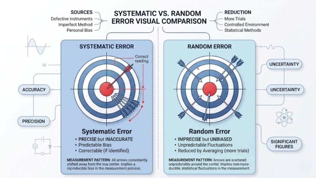
Systematic error is a consistent, reproducible deviation of all measurements from the true value in the same direction. Every reading is shifted — either all too high or all too low — by roughly the same amount. Because the bias is consistent, taking more readings does not help. The average of one hundred biased readings is still biased.
This is the defining characteristic that makes systematic error particularly dangerous: it is invisible to the standard statistical tools (like averaging) that reduce random error.
Physical Origins
Systematic errors arise from several distinct sources:
Instrument error: The instrument itself is miscalibrated, worn, or damaged. A ruler with a worn end gives every length measurement slightly too short. A thermometer whose markings have been printed slightly off-scale gives every temperature reading shifted by a fixed amount.
Zero error: A specific type of instrument error. The instrument does not read zero when the measured quantity is zero. A Vernier caliper with a positive zero error reads 0.04 cm when the jaws are fully closed — every subsequent measurement will be 0.04 cm too high.
\[ \text{Corrected Reading} = \text{Observed Reading} – \text{Zero Error} \]
Environmental error: External conditions — temperature, humidity, air pressure, magnetic fields — systematically affect the measurement. A steel metre ruler expands with temperature, making every measurement slightly longer on a hot day than on a cold one. A galvanometer used near a strong external magnetic field will show systematic deflection even with no current through it.
Methodological error: The experimental procedure itself introduces a consistent bias. In a pendulum experiment, measuring the string length from the support to the top of the bob instead of to the bob’s centre of mass consistently underestimates the true pendulum length by half the bob’s diameter — a fixed error that propagates into every calculated value of g.
Personal error (observer bias): Individual habits of observation that affect results consistently. A student who habitually reads a meniscus from slightly above eye level will consistently record volumes that are too high.
Real-World Example
In an experiment to measure the acceleration due to gravity using a simple pendulum, a student measures the length of the pendulum from the pivot to the top of the bob, instead of to its centre of mass. The bob has a radius of 1.2 cm. Every length measurement is 1.2 cm too short. Since \( g \propto L \), every calculated value of g will also be systematically low. Repeating the experiment fifty times does not fix this — the methodological error is reproduced faithfully every time.
How to Minimize Systematic Error
- Calibrate all instruments before use. Compare the instrument against a known standard. If the instrument reads a standard mass of 100.0 g as 98.5 g, the systematic offset is −1.5 g for every reading.
- Check and correct for zero error. For every instrument with a zero point — Vernier caliper, screw gauge, ammeter, spring balance — check the reading when the measured quantity is zero. Apply the correction formula.
- Use established, verified experimental procedures. Methodological errors are eliminated by following procedures that have been developed and tested specifically to avoid known biases.
- Control environmental conditions. Conduct temperature-sensitive experiments in a controlled environment. Shield galvanometers from stray magnetic fields. Allow instruments to acclimatize to the lab temperature before use.
- Use a different method to measure the same quantity. If two independent methods give the same result, systematic errors specific to one method are unlikely to be present in both. A persistent discrepancy between methods is a strong signal of systematic error in one of them.
Error 2: Random Error
What It Is
Random error is the unpredictable, non-reproducible variation in measurements taken under apparently identical conditions. Unlike systematic error, random errors do not consistently push the result in one direction — they scatter readings on both sides of the true value. Some readings will be slightly high, some slightly low and the distribution of readings around the true value follows a pattern that, for well-behaved experiments, approximates a normal (Gaussian) distribution.
Because random errors are genuinely random in direction, they can be reduced by averaging: the positive deviations and negative deviations partially cancel when the mean is computed. More readings mean a better-estimated mean, with the uncertainty in the mean decreasing as \( 1/\sqrt{n} \) where \( n \) is the number of readings.
Physical Origins
Limitations of human observation: Reading a scale involves estimating between the finest graduations. Different moments of reading produce slightly different estimates. Even the same observer, reading immediately twice, will produce slightly different results.
Genuine variability in the physical system: Some systems are intrinsically variable. The exact moment a pendulum completes an oscillation is not perfectly reproducible from cycle to cycle — there are microscopic variations in air resistance, tiny changes in amplitude and slight variations in the pivot condition.
Environmental fluctuations: Small, uncontrolled changes in temperature, air currents, vibration and electrical noise introduce fluctuations into measurements that cannot be fully controlled.
Instrument resolution limit: At the finest scale of any instrument, there is inherent imprecision in reading between the smallest divisions. This contributes a component of random scatter to all readings.
Mathematical Treatment
The mean value from \( n \) measurements is the best estimate of the true value:
\[ \bar{x} = \frac{1}{n}\sum_{i=1}^{n} x_i \]
The mean absolute error quantifies the spread of readings:
\[ \overline{\Delta x} = \frac{1}{n}\sum_{i=1}^{n} |x_i – \bar{x}| \]
The result is reported as:
\[ x = \bar{x} \pm \overline{\Delta x} \]
The uncertainty in the mean decreases with more readings. This is why timing 20 oscillations of a pendulum and dividing by 20 gives a much more reliable period than timing a single oscillation — the reaction time error, which behaves like random error, becomes \( \frac{1}{20} \) of its single-measurement value.
Real-World Example
A student times 10 oscillations of a simple pendulum using a digital stopwatch (LC = 0.01 s). The readings are: 14.23, 14.31, 14.18, 14.27, 14.22 seconds. The mean is 14.24 s, giving a period of 1.424 s. The scatter of ±0.07 s across readings reflects random error — reaction time variations, slight differences in the start and stop positions and air current fluctuations.
If the student had instead timed 50 oscillations five times, the uncertainty in each reading would be spread over a much larger interval, making the percentage effect of reaction time much smaller.
How to Minimize Random Error
- Take more readings and compute the mean. The uncertainty in the mean scales as \( 1/\sqrt{n} \). Doubling the number of readings reduces the random error in the mean by a factor of \( \sqrt{2} \approx 1.41 \). Ten times the readings gives \( \sqrt{10} \approx 3.16 \) times better precision.
- Time multiple events and divide. For periodic phenomena, always time \( n \) complete cycles and divide by \( n \). The reaction time error, which is constant per measurement, becomes \( n \) times smaller as a fraction of the total measured time.
- Use more precise instruments. An instrument with a smaller least count introduces less quantization uncertainty per reading.
- Reduce environmental disturbances. Use vibration-isolated benches for sensitive measurements. Shield experiments from air currents. Stabilize the power supply voltage in electrical experiments.
- Allow the system to reach equilibrium before reading. Wait for a thermometer to equilibrate with the liquid. Wait for a spring balance pointer to stop oscillating. A reading taken before equilibrium contributes a systematic-like component to what would otherwise be clean random error.
Error 3: Parallax Error
What It Is
Parallax error is a specific and extremely common form of systematic error caused by the incorrect positioning of the observer’s eye relative to the measuring scale. When the observer’s line of sight is not perpendicular to the scale at the point of measurement, the scale markings appear shifted relative to the pointer or liquid surface, producing a reading that is consistently too high or consistently too low depending on the angle of observation.
It is classified as a systematic error because a given observer with a fixed habitual viewing angle will produce the same offset in every reading.
Physical Origin
Consider a pointer that sits a small distance above the scale face — as is the case in almost every analogue meter. If the observer’s eye is above and to the left of the pointer, they see the pointer apparently pointing to a mark to the right of its true position. If the eye is above and to the right, the pointer appears to point to a mark to the left. Only when the eye is exactly level and directly in front of the pointer does the apparent position match the true position.
The same effect occurs when reading a ruler placed against an object: if the zero mark is not in contact with the object’s surface and the eye is not directly above the reading point, the apparent reading is shifted.
Real-World Examples
- Reading an ammeter or voltmeter from an angle causes the pointer to appear shifted toward or away from the reader, giving a biased reading.
- Reading a measuring cylinder from above makes the meniscus appear higher than it is — the volume reading is too large.
- Reading a thermometer from below makes the column appear shorter — the temperature reading is too low.
How to Minimize Parallax Error
- Position the eye directly level with and perpendicular to the scale. This is the fundamental fix. The line of sight must pass through the reading point at right angles to the scale surface.
- Use the mirror strip on analogue meters. Most laboratory ammeters and voltmeters have a mirror strip behind the scale. When the observer’s reflection in the mirror is directly behind the pointer — when pointer and reflection appear as one — the line of sight is perpendicular and parallax is eliminated.
- Use digital instruments where possible. Digital displays present no parallax problem — the reading is unambiguous regardless of viewing angle.
- Bring the scale as close as possible to the object being measured. In ruler measurements, the zero graduation on the ruler should be in contact with the object’s surface, not elevated above it.
- Use a set square or plumb line. In situations where the eye level is difficult to judge, a set square held against the scale ensures the line of sight is perpendicular.
Error 4: Instrumental Error (Least Count and Calibration Error)
What It Is
Instrumental error encompasses two related but distinct problems: the finite resolution of any measuring instrument (expressed as its least count) and the possible miscalibration of the instrument’s scale against the true standard.
Every instrument can only resolve differences down to its least count. A reading that falls between two graduations must be estimated — and that estimate introduces an irreducible uncertainty. This is sometimes called the quantization error or resolution error of the instrument.
Calibration error occurs when the instrument’s scale does not accurately represent the physical quantity it claims to measure — typically because the instrument has drifted from its original calibration, has been damaged, or was manufactured to a lower standard.
The Least Count and Its Role in Error
For a direct-reading instrument, the absolute error due to the instrument alone is taken as:
\[ \Delta x_\text{instrument} = \pm \frac{1}{2} \times \text{Least Count} \]
or more conservatively (and more commonly in school-level physics):
\[ \Delta x_\text{instrument} = \pm \text{Least Count} \]
This tells you the minimum possible error you can have in a single reading with that instrument — even if your technique is perfect.
For a Vernier caliper with LC = 0.01 cm: \[ \Delta x_\text{min} = \pm 0.01 \text{ cm} \]
For a screw gauge with LC = 0.01 mm: \[ \Delta x_\text{min} = \pm 0.01 \text{ mm} \]
This is why instrument choice matters. Measuring a wire diameter with a ruler (LC = 1 mm) when the diameter is approximately 0.4 mm is not just imprecise — it is meaningless. The least count is larger than the quantity being measured.
Propagation into Derived Quantities
When a derived quantity is calculated from measured values, the instrumental errors propagate according to the error propagation rules:
For \( Z = \frac{A^p \cdot B^q}{C^r} \):
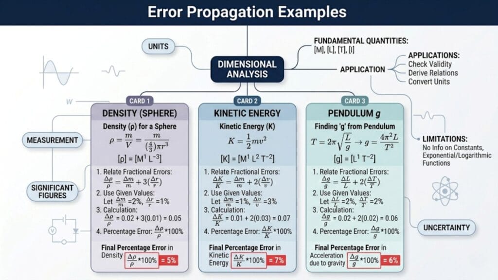
\[ \frac{\Delta Z}{Z} = p\frac{\Delta A}{A} + q\frac{\Delta B}{B} + r\frac{\Delta C}{C} \]
A small least count error in a base measurement becomes amplified when that measurement is raised to a power. The error in a volume calculated from a radius measurement is three times the relative error in the radius — because volume scales as \( r^3 \).
Learn more about Propagation of Errors in Physics Calculations: Rules, Formulas & Examples
Real-World Example
A student measures the radius of a sphere with a Vernier caliper: \( r = 2.53 \pm 0.01 \) cm. The volume is:
\[ V = \frac{4}{3}\pi r^3 \]
\[ \frac{\Delta V}{V} = 3 \times \frac{\Delta r}{r} = 3 \times \frac{0.01}{2.53} \approx 3 \times 0.00395 \approx 1.19\% \]
A 0.4% error in radius becomes a 1.2% error in volume — amplified by the cube exponent.
How to Minimize Instrumental Error
- Choose the instrument with the appropriate least count. Match the instrument’s precision to the precision actually required. Using a screw gauge (LC = 0.01 mm) for an object 15 cm long is inconvenient and unnecessary. Using a ruler (LC = 1 mm) for a wire 0.5 mm in diameter is inadequate.
- Calibrate instruments against verified standards before use. Compare the instrument’s reading against a certified reference standard and apply a correction factor if needed.
- Use instruments in good repair. Worn jaws on a Vernier caliper, a bent pointer on an ammeter, or a damaged scale on a ruler all introduce calibration errors that simple zero-error correction cannot fix.
- Be aware of which measurement dominates the error budget. When multiple measurements contribute to a derived quantity, identify which one contributes most to the final error. Improve the precision of that measurement first — improving the others has diminishing returns.
Error 5: Personal Error (Human Error)
What It Is
Personal error, sometimes called human error or observer error, refers to errors arising from the individual characteristics and habits of the person making the measurement. It is distinct from gross error (which is an outright mistake or blunder) because personal errors are often unconscious, habitual and systematic within a given observer’s measurements.
Personal errors straddle the line between systematic and random error:
- Systematic personal error: A consistent habit — always reading a scale from the same angle, always pressing a stopwatch with the same delay — produces a consistent offset in the same direction.
- Random personal error: Slight variations in attention, estimation and timing produce scatter in repeated readings.
Physical Origins and Common Forms
Anticipation error (timing experiments): When timing an oscillating pendulum, a student who watches the pendulum and anticipates the return to the extreme position will stop the watch slightly early. This gives a period that is consistently shorter than the true value.
Scale interpolation bias: Estimating the position of a pointer between two scale divisions involves judgment. Some students consistently round toward the nearest major division; others consistently estimate a higher fraction. This produces a systematic shift in all readings by that observer.
End-digit preference: Some observers show a strong preference for certain final digits — particularly 0 and 5 — when estimating between graduations. This creates a non-uniform distribution of readings that does not reflect the true physical distribution.
Fatigue and attention errors: Over a long series of measurements, concentration lapses. Later readings in a session may be less careful than earlier ones, introducing a time-dependent random component.
Handedness and viewing angle: An observer’s dominant hand affects how they hold and position instruments. A right-handed student may habitually view a scale from a slightly rightward angle, creating a consistent parallax offset specific to that individual.
Real-World Example
Two students measure the time period of the same pendulum independently. Student A gets \( T = 1.87 \pm 0.03 \) s and Student B gets \( T = 1.94 \pm 0.04 \) s. The discrepancy (0.07 s) is larger than the stated uncertainty of either measurement, suggesting a systematic personal error — most likely in timing technique. Student A may be stopping the watch early (anticipation), while Student B may be stopping it late (delayed reaction). The actual period is somewhere between the two.
How to Minimize Personal Error
- Use automatic or electronic triggering wherever possible. Replace manual stopwatch operation with light-gate timers or electronic sensors. Remove human reaction time from the measurement chain entirely.
- Practice the reading technique before recording data. Take practice readings without recording them until the technique is consistent. Familiarity with the instrument reduces the variability of estimation.
- Have readings taken and verified by a second observer. If two independent observers consistently agree, the personal error of each is likely small. Persistent disagreement reveals personal error in one or both.
- Be explicitly aware of habitual biases. If you know you tend to read a scale from slightly above eye level, consciously correct for this. Named biases are easier to control than unnamed ones.
- Use blind reading where feasible. In some experimental setups, the observer can be shielded from seeing the previous reading before taking the next one, preventing unconscious anchoring to earlier values.
- Time multiple events. For periodic phenomena, timing 20 or 50 cycles and dividing reduces the relative contribution of reaction time — a major source of personal error in timing — by a factor of 20 or 50.
Summary: Five Errors, Their Origins and Minimization Strategies
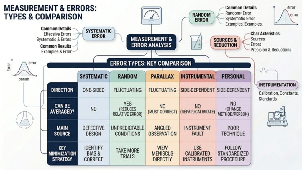
| Error Type | Category | Direction | Averaged Away? | Best Minimization Strategy |
| Systematic Error | Systematic | Consistent, one direction | No | Calibrate instruments; check zero error; verify method |
| Random Error | Random | Both directions, unpredictable | Yes | Take more readings; time multiple events; use precise instruments |
| Parallax Error | Systematic | Depends on viewing angle | No | Eye perpendicular to scale; use mirror strip; use digital instruments |
| Instrumental Error | Systematic/Fundamental | Fixed by LC and calibration | No | Choose appropriate instrument; calibrate; be aware of LC limits |
| Personal Error | Both | Consistent or scattered | Partially | Use automatic triggers; practice technique; second observer |
How Errors Combine in a Complete Experiment
In any real experiment, multiple error sources are present simultaneously. The total error in a final derived quantity is not the sum of all individual errors — that would overestimate the uncertainty. For independent random errors, they combine in quadrature:
\[ \Delta Z_\text{total} = \sqrt{(\Delta Z_1)^2 + (\Delta Z_2)^2 + (\Delta Z_3)^2 + \cdots} \]
For systematic errors that are known in sign and magnitude, they are added algebraically. For worst-case analysis (most conservative approach, used in school-level physics):
\[ \Delta Z_\text{total} = \Delta Z_1 + \Delta Z_2 + \Delta Z_3 + \cdots \]
This worst-case addition is what the CBSE board exam and JEE/NEET error propagation formulas use:
\[ \frac{\Delta Z}{Z} = p\frac{\Delta A}{A} + q\frac{\Delta B}{B} + r\frac{\Delta C}{C} \]
The important practical skill is identifying which single error source dominates the total. Improving a measurement that contributes 0.1% to the total error while another contributes 3% is a waste of effort. Always tackle the largest error source first.
Learn more about Measurement Uncertainty in Physics: What It Is and Why It Always Exists
Errors in the Context of Accuracy and Precision
These two concepts are closely related to the error discussion but have distinct meanings:
Accuracy describes how close the measured value is to the true value. It is limited primarily by systematic errors. High systematic error means low accuracy.
Precision describes how reproducible the measurements are — how tightly they cluster together regardless of where that cluster sits. It is limited primarily by random error and instrumental error. High random error means low precision.
A measurement can be precise without being accurate (all readings cluster tightly around a wrong value — systematic error is large) and it can be accurate without being precise (readings scatter widely but average to the correct value — random error is large, systematic error is small).
The ideal measurement is both: high precision (low random error) and high accuracy (low systematic error).
Learn more about Accuracy vs Precision in Physics: Definition, Difference & Real-World Examples
Why This Understanding Matters for Exams
For CBSE board exams, errors appear in two forms: 3-mark short-answer questions defining and distinguishing error types and 2-to-3-mark numerical questions on percentage error calculation. Both are straightforward if the conceptual framework is solid.
For JEE Main and NEET, error propagation numericals are the primary format. The question gives a formula for a derived quantity, states percentage errors in each measured variable and asks for the percentage error in the result. These are solved in two lines using the general propagation formula — but only if the student understands why each term in that formula corresponds to an actual physical error source.
A student who understands measurement error at the level of this article will find both the conceptual and numerical questions straightforward. A student who has only memorized the formulas without the physical understanding will struggle whenever the question is phrased in a slightly unfamiliar way.
Learn more about NEET Physics: Units & Measurements – Chapter Notes with MCQs
Conclusion
Error in physics measurement is not something to be embarrassed about or papered over. It is something to be understood, named, quantified and managed. The five error types covered in this article — systematic, random, parallax, instrumental and personal — cover the full landscape of what can go wrong between a physical quantity and the number written in a lab notebook.
Each error type has a distinct physical origin. Each requires a distinct strategy to minimize. And each has a distinct mathematical signature that appears in how measurements scatter, how they compare to the true value and how they propagate into calculated results.
The experimenter who walks into a lab knowing all of this is not just more likely to get the right answer. They are doing physics — understanding the measurement process at a level that turns data into knowledge.
Frequently Asked Questions
What is the difference between systematic error and random error?
Systematic error shifts all measurements consistently in one direction by roughly the same amount. It cannot be reduced by averaging. Random error causes measurements to scatter unpredictably in both directions around the true value. It can be reduced by taking more readings and averaging. A biased thermometer with the wrong calibration produces systematic error; the slight variability in stopwatch readings from one trial to the next is random error.
Can systematic error be negative?
Yes. Systematic error can be positive (all readings too high) or negative (all readings too low). The sign depends on the direction of the bias. A worn-down ruler gives negative systematic error in length measurements (readings too short). A Vernier caliper with positive zero error gives positive systematic error (readings too high).
What is the easiest way to detect systematic error in an experiment?
The clearest signal of systematic error is a consistent discrepancy between results from two different measurement methods applied to the same quantity. If a distance measured with a ruler consistently differs from the same distance measured with a Vernier caliper by more than the combined random errors of both methods, systematic error is present in at least one of the methods.
How does parallax error differ from personal error?
Parallax error has a specific physical mechanism — the misalignment of the line of sight with the scale — and can be precisely eliminated by correct eye positioning or using a mirror strip. Personal error is a broader category covering all observer-dependent biases, including viewing angle habits, timing anticipation, scale interpolation preferences and attention lapses. Parallax error is one form of personal error, but personal error includes much more.
Why can’t random errors be completely eliminated?
Random errors arise from genuinely uncontrollable fluctuations at the limit of the measurement process — human estimation between scale divisions, microscopic environmental variations and quantum-level noise in the physical system. These cannot be eliminated because they are inherent to the act of measurement at finite resolution. They can only be reduced — by averaging more readings, using more precise instruments and controlling environmental conditions better.
Is zero error a systematic or instrumental error?
Zero error is both. It is a form of instrumental error because it arises from the instrument itself — the zero point of the scale does not correspond to the zero of the physical quantity. It is also a systematic error because it shifts every reading consistently in the same direction by the same amount. It is corrected by subtracting the zero error (with its sign) from every observed reading.
What does it mean to say an error “propagates” into a calculated result?
When a physical quantity is calculated from two or more measured values, the uncertainties in those measured values carry through into the calculated result. This carrying-through is called propagation. For example, if density is calculated as mass divided by volume and both mass and volume have percentage errors, those errors propagate into the calculated density. The general formula \( \Delta Z/Z = p\Delta A/A + q\Delta B/B + r\Delta C/C \) quantifies exactly how much each measured error contributes to the final result’s uncertainty.
Leave a Comment