

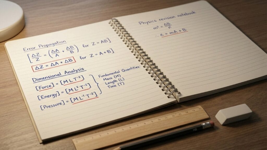
Introduction
The night before a board exam, most students do not want to re-read the textbook. They want a single reliable place where every formula they need is organized, clearly explained and ready to use. This article is built for exactly that moment — and for every revision session leading up to it.
Units and Measurements is a chapter that rewards formula fluency. Unlike chapters that require lengthy derivations or conceptual essays, the questions here are almost always short and numerical. Know the right formula, apply it correctly, write the answer with proper units — done. The marks are there for students who have prepared this chapter properly and consistently lost by those who assumed they knew it well enough without ever sitting down to consolidate it.
Every formula in this article comes with a clear explanation of what it means, what each symbol stands for and a worked example where the concept benefits from one. This is not a bare formula sheet. It is a formula guide — the kind you can actually learn from, not just copy.
How to Use This Article
The formulas are organized into six sections, matching the natural structure of the chapter:
- Units and Measurement Basics
- Significant Figures
- Dimensional Formulas
- Dimensional Analysis — Applications
- Errors in Measurement
- Measuring Instruments — Least Count
Work through each section in order on your first read. On subsequent revision passes, jump directly to whichever section needs more attention. The worked examples are placed where the formula application is non-obvious — skip them only if the formula feels fully clear.
Section 1: Units and Measurement Basics
Formula 1.1 — Relationship Between Numerical Value and Unit
\[ n_1 u_1 = n_2 u_2 \]
Where:
- \( n_1, n_2 \) = numerical values of the same physical quantity in two different unit systems
- \( u_1, u_2 \) = the corresponding units
What it means: The physical quantity itself does not change when you change the unit. If the unit is made larger, the numerical value gets smaller and vice versa. Their product stays constant.
Example: 1 km = 1000 m. Here \( n_1 = 1 \), \( u_1 = \text{km} \), \( n_2 = 1000 \), \( u_2 = \text{m} \). The distance is the same regardless of which pair you write.
Formula 1.2 — General Unit Conversion Using Dimensional Method
\[ n_2 = n_1 \left[\frac{M_1}{M_2}\right]^a \left[\frac{L_1}{L_2}\right]^b \left[\frac{T_1}{T_2}\right]^c \]
Where:
- \( n_1 \) = numerical value in the original system
- \( n_2 \) = numerical value in the new system
- \( M_1, L_1, T_1 \) = base units (mass, length, time) of the original system
- \( M_2, L_2, T_2 \) = base units of the new system
- \( a, b, c \) = dimensional exponents of the physical quantity (from its dimensional formula)
What it means: To convert any physical constant or quantity between unit systems, substitute the known base unit values of each system and the dimensional exponents of the quantity. The formula handles the rest automatically.
Example: To convert the value of G from CGS to SI:
- \( [G] = M^{-1}L^3T^{-2} \), so \( a = -1, b = 3, c = -2 \)
- \( n_1 = 6.67 \times 10^{-8} \) (CGS value)
- \( M_1/M_2 = 1\text{ g}/1\text{ kg} = 10^{-3} \), \( L_1/L_2 = 1\text{ cm}/1\text{ m} = 10^{-2} \), \( T_1/T_2 = 1 \)
\[ n_2 = 6.67 \times 10^{-8} \times (10^{-3})^{-1} \times (10^{-2})^3 \times (1)^{-2} \]
\[ = 6.67 \times 10^{-8} \times 10^3 \times 10^{-6} = 6.67 \times 10^{-11} \]
Result: \( G = 6.67 \times 10^{-11} \) N m² kg⁻² in SI.
Learn more about How to Convert Units in Physics: Step-by-Step with Solved Examples
Section 2: Significant Figures
Formula 2.1 — Rounding Rule for Multiplication and Division
\[ \text{Significant figures in result} = \text{Fewest significant figures among all inputs} \]
Example: \( 4.56 \times 1.4 = 6.384 \rightarrow \text{rounded to } 6.4 \) (2 sig figs, matching 1.4)
Formula 2.2 — Rounding Rule for Addition and Subtraction
\[ \text{Decimal places in result} = \text{Fewest decimal places among all inputs} \]
Example: \( 123.4 + 5.67 + 0.012 = 129.082 \rightarrow \text{rounded to } 129.1 \) (1 decimal place, matching 123.4)
Critical distinction: Addition and subtraction use decimal places — not significant figures. This is the most common source of confusion in this section and appears regularly in board exam multiple-choice questions.
Learn more about How to Find Significant Figures: Rules, Examples & Common Mistakes
Section 3: Dimensional Formulas
These are not formulas in the algebraic sense — they are systematic expressions of how each physical quantity is built from the base dimensions M (mass), L (length), T (time), A (electric current), K (temperature) and others.
Formula 3.1 — The General Dimensional Expression
\[ [Q] = M^a L^b T^c A^d K^e \cdots \]
Where \( a, b, c, d, e \) are rational numbers (integers in most cases) determined by the defining equation of the quantity Q.
Complete Dimensional Formula Table
| Physical Quantity | Defining Relation | Dimensional Formula |
| Area | length × breadth | \( [L^2] \) |
| Volume | length × breadth × height | \( [L^3] \) |
| Velocity / Speed | displacement ÷ time | \( [LT^{-1}] \) |
| Acceleration | velocity ÷ time | \( [LT^{-2}] \) |
| Force | mass × acceleration | \( [MLT^{-2}] \) |
| Momentum | mass × velocity | \( [MLT^{-1}] \) |
| Impulse | force × time | \( [MLT^{-1}] \) |
| Work / Energy | force × displacement | \( [ML^2T^{-2}] \) |
| Kinetic Energy | \( \frac{1}{2}mv^2 \) | \( [ML^2T^{-2}] \) |
| Potential Energy | mgh | \( [ML^2T^{-2}] \) |
| Torque | force × perpendicular distance | \( [ML^2T^{-2}] \) |
| Power | work ÷ time | \( [ML^2T^{-3}] \) |
| Pressure / Stress | force ÷ area | \( [ML^{-1}T^{-2}] \) |
| Density | mass ÷ volume | \( [ML^{-3}] \) |
| Gravitational Constant G | \( F = Gm_1m_2/r^2 \) | \( [M^{-1}L^3T^{-2}] \) |
| Angular Velocity | angle ÷ time | \( [T^{-1}] \) |
| Frequency | cycles ÷ time | \( [T^{-1}] \) |
| Angular Acceleration | angular velocity ÷ time | \( [T^{-2}] \) |
| Moment of Inertia | mass × (radius)² | \( [ML^2] \) |
| Angular Momentum | moment of inertia × angular velocity | \( [ML^2T^{-1}] \) |
| Surface Tension | force ÷ length | \( [MT^{-2}] \) |
| Coefficient of Viscosity η | from Newton’s viscosity law | \( [ML^{-1}T^{-1}] \) |
| Spring Constant k | force ÷ displacement | \( [MT^{-2}] \) |
| Planck’s Constant h | energy ÷ frequency | \( [ML^2T^{-1}] \) |
| Boltzmann Constant k_B | energy ÷ temperature | \( [ML^2T^{-2}K^{-1}] \) |
| Universal Gas Constant R | energy ÷ (mol × temperature) | \( [ML^2T^{-2}K^{-1}mol^{-1}] \) |
| Charge | current × time | \( [AT] \) |
| Electric Potential | work ÷ charge | \( [ML^2T^{-3}A^{-1}] \) |
| Resistance | potential ÷ current | \( [ML^2T^{-3}A^{-2}] \) |
| Electric Field | force ÷ charge | \( [MLT^{-3}A^{-1}] \) |
| Capacitance | charge ÷ potential | \( [M^{-1}L^{-2}T^4A^2] \) |
| Magnetic Field B | from \( F = qvB \) | \( [MT^{-2}A^{-1}] \) |
| Magnetic Flux | B × area | \( [ML^2T^{-2}A^{-1}] \) |
| Inductance L | from \( V = L\frac{dI}{dt} \) | \( [ML^2T^{-2}A^{-2}] \) |
| Permittivity \( \varepsilon_0 \) | from Coulomb’s law | \( [M^{-1}L^{-3}T^4A^2] \) |
| Permeability \( \mu_0 \) | from Biot–Savart law | \( [MLT^{-2}A^{-2}] \) |
Pairs of Quantities Sharing the Same Dimensional Formula
Board exams and competitive exams both test this. Know these pairs cold:
| Dimensional Formula | Quantities That Share It |
| \( [ML^2T^{-2}] \) | Work, Energy, Torque, Heat |
| \( [MLT^{-1}] \) | Momentum, Impulse |
| \( [MT^{-2}] \) | Surface Tension, Spring Constant |
| \( [ML^{-1}T^{-2}] \) | Pressure, Stress, Bulk Modulus, Young’s Modulus |
| \( [ML^2T^{-1}] \) | Angular Momentum, Planck’s Constant |
| \( [T^{-1}] \) | Frequency, Angular Velocity |
Learn more about What Is Dimensional Formula? Derivation, Applications & Limitations
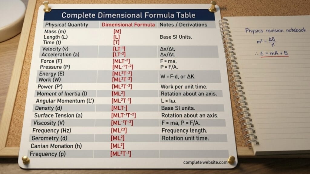
Section 4: Dimensional Analysis — Key Formulas and Applications
Formula 4.1 — Principle of Dimensional Homogeneity
\[ [LHS] = [RHS] \]
Every term on both sides of a physically valid equation must have identical dimensional formulas. Every term being added or subtracted within the equation must also share the same dimensions.
Application — Checking an equation:
Check whether \( v^2 = u^2 + 2as \) is dimensionally valid.
\[ [v^2] = L^2T^{-2} \] \[ [u^2] = L^2T^{-2} \] \[ [2as] = LT^{-2} \times L = L^2T^{-2} \]
All terms carry \( [L^2T^{-2}] \). The equation is dimensionally homogeneous and therefore potentially valid.
Formula 4.2 — Deriving a Relation by Dimensional Analysis (Method of Undetermined Exponents)
If a quantity \( Q \) depends on quantities \( A \), \( B \) and \( C \):
\[ Q = k \cdot A^x B^y C^z \]
Where \( k \) is a dimensionless constant and \( x, y, z \) are unknown exponents. Taking dimensions of both sides and comparing exponents of M, L and T gives a system of three equations that determines \( x, y, z \).
Example — Time period of a simple pendulum:
Assume \( T \propto l^x \cdot m^y \cdot g^z \)
\[ [T] = [L]^x [M]^y [LT^{-2}]^z \] \[ T^1 = M^y L^{x+z} T^{-2z} \]
Comparing:
- M: \( y = 0 \)
- T: \( -2z = 1 \Rightarrow z = -\frac{1}{2} \)
- L: \( x + z = 0 \Rightarrow x = \frac{1}{2} \)
\[ T = k\sqrt{\frac{l}{g}} \]
Dimensional analysis gives the form. The constant \( k = 2\pi \) comes from full theory.
Learn more about Dimensional Analysis Made Easy: Method, Rules and Practice Problems
Section 5: Errors in Measurement
This section has the highest formula density and generates the most board exam numerical questions. Every formula below has appeared in CBSE exams. Learn them as a set — they build on each other logically.
Formula 5.1 — Mean (Average) Value
\[ \bar{x} = \frac{x_1 + x_2 + x_3 + \cdots + x_n}{n} \]
The best estimate of the true value from \( n \) repeated measurements.
Formula 5.2 — Absolute Error of Each Reading
\[ \Delta x_i = |x_i – \bar{x}| \]
The magnitude of deviation of each individual reading from the mean. Always positive — use absolute value.
Formula 5.3 — Mean Absolute Error
\[ \overline{\Delta x} = \frac{\Delta x_1 + \Delta x_2 + \cdots + \Delta xn}{n} = \frac{\sum{i=1}^{n} \Delta x_i}{n} \]
The average of all individual absolute errors. This is the uncertainty you report alongside your measured value.
Formula 5.4 — Reporting the Result
\[ x = \bar{x} \pm \overline{\Delta x} \]
This tells the reader: the true value lies somewhere in the interval \( [\bar{x} – \overline{\Delta x},\ \bar{x} + \overline{\Delta x}] \).
Formula 5.5 — Relative (Fractional) Error
\[ \delta_r = \frac{\overline{\Delta x}}{\bar{x}} \]
A dimensionless ratio expressing error as a fraction of the measured value. Useful for comparing the precision of measurements of different quantities.
Formula 5.6 — Percentage Error
\[ \delta_\% = \frac{\overline{\Delta x}}{\bar{x}} \times 100\% \]
Percentage error is relative error expressed as a percentage. This is the form most commonly required in board exam answers.
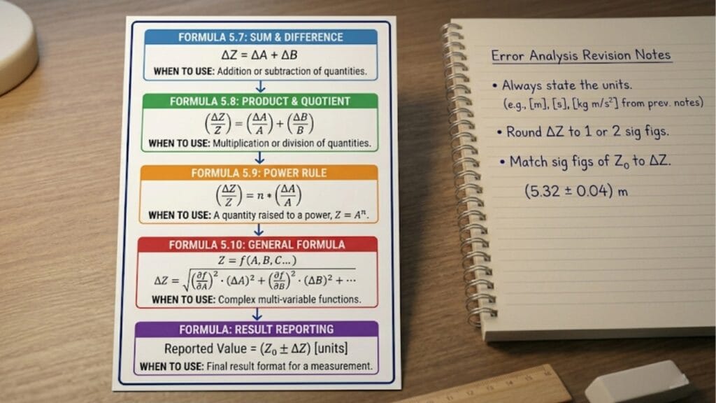
Formula 5.7 — Error Propagation: Sum or Difference
For \( Z = A + B \) or \( Z = A – B \):
\[ \Delta Z = \Delta A + \Delta B \]
Key point: Errors always add, even in subtraction. Uncertainty is always positive — the worst case is when both individual errors act in the same direction, which gives the maximum possible error in the result regardless of the sign of the operation.
Example: If \( A = 5.0 \pm 0.1 \) cm and \( B = 3.0 \pm 0.2 \) cm:
\[ Z = A – B = 2.0 \text{ cm}, \quad \Delta Z = 0.1 + 0.2 = 0.3 \text{ cm} \]
Result: \( Z = 2.0 \pm 0.3 \) cm
Formula 5.8 — Error Propagation: Product or Quotient
For \( Z = A \times B \) or \( Z = \frac{A}{B} \):
\[ \frac{\Delta Z}{Z} = \frac{\Delta A}{A} + \frac{\Delta B}{B} \]
Relative errors add for products and quotients.
Example: If \( A = 10.0 \pm 0.2 \) and \( B = 5.0 \pm 0.1 \):
\[ \frac{\Delta Z}{Z} = \frac{0.2}{10.0} + \frac{0.1}{5.0} = 0.02 + 0.02 = 0.04 \]
\[ \% \text{ error in } Z = 4\% \]
Formula 5.9 — Error Propagation: Power of a Quantity
For \( Z = A^n \):
\[ \frac{\Delta Z}{Z} = |n| \cdot \frac{\Delta A}{A} \]
The relative error is multiplied by the absolute value of the exponent. This is why errors in squared or cubed quantities grow quickly.
Example: If the percentage error in the radius of a sphere is 2%, the percentage error in its volume \( V = \frac{4}{3}\pi r^3 \) is:
\[ \frac{\Delta V}{V} \times 100 = 3 \times 2\% = 6\% \]
Formula 5.10 — General Error Propagation Formula
For \( Z = \frac{A^p \cdot B^q}{C^r} \):
\[ \frac{\Delta Z}{Z} = p\frac{\Delta A}{A} + q\frac{\Delta B}{B} + r\frac{\Delta C}{C} \]
This is the master formula that handles every combination of products, quotients and powers in a single expression. Every board exam numerical on error analysis is an application of this formula.
Example: The kinetic energy \( KE = \frac{1}{2}mv^2 \). If the percentage error in mass is 1% and in velocity is 3%, find the percentage error in KE.
\[ \frac{\Delta KE}{KE} \times 100 = \frac{\Delta m}{m} \times 100 + 2 \times \frac{\Delta v}{v} \times 100 \]
\[ = 1\% + 2 \times 3\% = 1\% + 6\% = 7\% \]
Worked Example: Full Error Analysis Problem
This is the type of problem that appears in CBSE board exams as a 3-mark question.
Problem: Five successive measurements of the diameter of a wire are: 1.22, 1.25, 1.23, 1.27 and 1.23 mm. Find (a) mean diameter, (b) mean absolute error, (c) relative error, (d) percentage error and (e) express the result in the standard form.
Solution:
(a) Mean:
\[ \bar{d} = \frac{1.22 + 1.25 + 1.23 + 1.27 + 1.23}{5} = \frac{6.20}{5} = 1.24 \text{ mm} \]
(b) Absolute errors:
\[ \Delta d_1 = |1.22 – 1.24| = 0.02 \] \[ \Delta d_2 = |1.25 – 1.24| = 0.01 \] \[ \Delta d_3 = |1.23 – 1.24| = 0.01 \] \[ \Delta d_4 = |1.27 – 1.24| = 0.03 \] \[ \Delta d_5 = |1.23 – 1.24| = 0.01 \]
Mean absolute error:
\[ \overline{\Delta d} = \frac{0.02 + 0.01 + 0.01 + 0.03 + 0.01}{5} = \frac{0.08}{5} = 0.016 \approx 0.02 \text{ mm} \]
(c) Relative error:
\[ \delta_r = \frac{0.02}{1.24} \approx 0.016 \]
(d) Percentage error:
\[ \delta_\% = 0.016 \times 100 \approx 1.6\% \]
(e) Result:
\[ d = 1.24 \pm 0.02 \text{ mm} \]
Learn more about Absolute Error, Relative Error and Percentage Error: A Complete Guide
Learn more about Propagation of Errors in Physics Calculations: Rules, Formulas & Examples
Section 6: Measuring Instruments — Least Count Formulas
Formula 6.1 — Least Count of Vernier Caliper
\[ \text{LC} = 1 \text{ MSD} – 1 \text{ VSD} \]
Equivalently:
\[ \text{LC} = \frac{\text{Value of 1 main scale division}}{\text{Total number of Vernier scale divisions}} \]
Standard values:
- 10-division Vernier: LC = 1 mm ÷ 10 = 0.1 mm
- 20-division Vernier: LC = 1 mm ÷ 20 = 0.05 mm
- 50-division Vernier: LC = 1 mm ÷ 50 = 0.02 mm
Formula 6.2 — Reading of Vernier Caliper
\[ \text{Total Reading} = \text{MSR} + (\text{VSR} \times \text{LC}) \]
\[ \text{Corrected Reading} = \text{Total Reading} – \text{Zero Error} \]
Where:
- MSR = Main Scale Reading (in mm or cm)
- VSR = Vernier Scale Reading (number of the coinciding Vernier division)
- Zero Error is positive if the Vernier zero lies to the right of the main scale zero (jaws closed); negative if it lies to the left
Formula 6.3 — Pitch of Screw Gauge
\[ \text{Pitch} = \frac{\text{Distance moved by spindle}}{\text{Number of complete rotations}} \]
Standard pitch: 0.5 mm
Formula 6.4 — Least Count of Screw Gauge
\[ \text{LC} = \frac{\text{Pitch}}{\text{Number of circular scale divisions}} \]
Standard value: LC = 0.5 mm ÷ 50 = 0.01 mm
Formula 6.5 — Reading of Screw Gauge
\[ \text{Total Reading} = \text{Sleeve Reading} + (\text{CSR} \times \text{LC}) \]
\[ \text{Corrected Reading} = \text{Total Reading} – \text{Zero Error} \]
Where:
- Sleeve Reading = whole mm value visible + 0.5 mm if the half-mm mark is exposed
- CSR = Circular Scale Reading (number of the division aligned with the reference line)
Learn more about Least Count of Vernier Caliper and Screw Gauge: Formula & Calculation
Instrument Formula Quick Reference
| Formula | Vernier Caliper | Screw Gauge |
| Least Count | \( \frac{1\text{ MSD}}{n_{\text{VSD}}} \) | \( \frac{\text{Pitch}}{n_{\text{CSD}}} \) |
| Standard LC | 0.1 mm | 0.01 mm |
| Reading | MSR + VSR × LC | SR + CSR × LC |
| Correction | Observed − Zero Error | Observed − Zero Error |
| Zero error sign | Positive if Vernier zero right of main zero | Positive if circular zero below reference line |
Learn more about How to Read a Measuring Instrument Correctly: Tips for Physics Lab
Board Exam Formula Summary Table
This table consolidates every formula from this article into a single compact reference. Use it for the final revision pass the day before your exam.
| Formula | Expression | Used For |
| Quantity relation | \( n_1 u_1 = n_2 u_2 \) | Unit equivalence |
| Dimensional conversion | \( n_2 = n_1 [M_1/M_2]^a [L_1/L_2]^b [T_1/T_2]^c \) | Converting between unit systems |
| Multiplication/Division sig figs | Fewest significant figures rule | Rounding computed results |
| Addition/Subtraction sig figs | Fewest decimal places rule | Rounding sums/differences |
| Homogeneity | \( [LHS] = [RHS] \) | Verifying equations dimensionally |
| Mean | \( \bar{x} = \sum x_i / n \) | Best estimate from repeated readings |
| Absolute error | \( \Delta x_i = \|x_i – \bar{x}\| \) | Deviation of each reading from mean |
| Mean absolute error | \( \overline{\Delta x} = \sum \Delta x_i / n \) | Overall uncertainty of measurement |
| Result reporting | \( x = \bar{x} \pm \overline{\Delta x} \) | Final measurement statement |
| Relative error | \( \delta_r = \overline{\Delta x}/\bar{x} \) | Fractional uncertainty |
| Percentage error | \( \delta_\% = (\overline{\Delta x}/\bar{x}) \times 100 \) | Uncertainty as percentage |
| Error in sum/difference | \( \Delta Z = \Delta A + \Delta B \) | Adding or subtracting measurements |
| Error in product/quotient | \( \Delta Z/Z = \Delta A/A + \Delta B/B \) | Multiplying or dividing measurements |
| Error in power | \( \Delta Z/Z = \|n\| \cdot \Delta A/A \) | Raising a measurement to a power |
| General error formula | \( \Delta Z/Z = p(\Delta A/A) + q(\Delta B/B) + r(\Delta C/C) \) | Any combination of operations |
| Vernier LC | \( 1\text{ MSD}/n_{\text{VSD}} \) | Precision of Vernier caliper |
| Screw gauge LC | \( \text{Pitch}/n_{\text{CSD}} \) | Precision of screw gauge |
| Vernier reading | \( \text{MSR} + \text{VSR} \times \text{LC} – \text{ZE} \) | Reading the Vernier caliper |
| Screw gauge reading | \( \text{SR} + \text{CSR} \times \text{LC} – \text{ZE} \) | Reading the screw gauge |
Common Formula Application Mistakes
Knowing a formula is only half the job. Applying it correctly under exam pressure is the other half. These are the mistakes that turn correct formula knowledge into wrong answers.
Mistake 1 — Using the wrong rule for significant figures in addition. The rule for addition and subtraction is decimal places, not significant figures. If you apply the multiplication rule to a sum, you will get an answer that appears reasonable but is wrong. Board examiners are specifically looking for this distinction.
Mistake 2 — Forgetting the absolute value sign in error of a power. In \( \frac{\Delta Z}{Z} = |n| \cdot \frac{\Delta A}{A} \), the exponent must be taken as a positive number. If \( n = -2 \) (as in \( T^{-2} \)), the contribution to relative error is still \( 2 \times \frac{\Delta T}{T} \), not \( -2 \times \frac{\Delta T}{T} \). Errors are always additive.
Mistake 3 — Not checking zero error before instrument reading. In both the Vernier caliper and screw gauge reading formulas, the correction step is:
\[ \text{Corrected Reading} = \text{Observed Reading} – \text{Zero Error} \]
A positive zero error must be subtracted. A negative zero error, when subtracted, effectively adds. Students who flip the sign consistently lose marks on instrument reading questions.
Mistake 4 — Treating the coinciding Vernier division as a length measurement. The VSR in the Vernier reading formula is a count of divisions — it is a pure number. It is not a length in mm. Multiply this number by the least count to get the fractional part of the reading in mm.
Mistake 5 — Applying dimensional analysis to check equations involving trigonometric functions. The argument of a trigonometric function must be dimensionless. If a proposed formula has \( \sin(vt) \) where \( v \) is velocity and \( t \) is time, the argument \( vt \) has dimensions of length — not dimensionless. That formula fails immediately and cannot be correct. This principle is itself tested in board exams.
Conclusion
Formulas without understanding are fragile — they break under unfamiliar question formats. Formulas with understanding are durable — they hold up even when the question is phrased in a way you have never seen before.
Every formula in this article has been presented with its meaning, its variables defined and its application demonstrated. The goal is not to hand you a list to memorize but to give you a set of tools you understand well enough to deploy correctly under pressure.
Read through this article twice before your board exam. On the second pass, cover the right-hand side of the summary table and write out each formula from memory. Any formula you cannot reproduce cleanly without looking is the one that needs another hour of attention. That targeted revision is far more efficient than re-reading the entire chapter.
Learn more about Units & Measurements One-Shot Revision: Complete Chapter for JEE & NEET
Frequently Asked Questions
Which formulas from Units and Measurements are most important for CBSE board exams?
The error propagation formulas — particularly the general formula \( \Delta Z/Z = p(\Delta A/A) + q(\Delta B/B) + r(\Delta C/C) \) — are the most frequently tested numerically. Dimensional formula derivations and the principle of homogeneity are the most frequently tested conceptually. All formulas for significant figures, least count and the dimensional conversion formula are also directly testable.
How do I remember all the dimensional formulas for board exams?
Derive them from the defining equation of each quantity rather than memorizing them as standalone facts. Once you can derive force as \( [MLT^{-2}] \) from \( F = ma \), the same logic extends to every other derived quantity. Derivation is faster under exam pressure and cannot fail on unfamiliar quantities the way memorization can.
What is the difference between absolute error and mean absolute error?
Absolute error (\( \Delta x_i \)) is the deviation of a single reading from the mean. Mean absolute error (\( \overline{\Delta x} \)) is the average of all individual absolute errors across all readings. The mean absolute error is what you report as the uncertainty of the measurement — it represents the overall reliability of the measurement process.
Why do errors add even when subtracting two quantities?
Because error represents uncertainty — an always-positive range within which the true value lies. When subtracting \( B \) from \( A \), the worst-case deviation in the result occurs when \( A \) is at its maximum and \( B \) is at its minimum, or vice versa. Both scenarios give a deviation of \( \Delta A + \Delta B \) from the calculated result. The sign of the arithmetic operation does not change this.
How many significant figures should I report in a board exam answer?
Report the result to the same number of significant figures as the least precise input (for multiplication/division) or the same number of decimal places as the least precise input (for addition/subtraction). If the question specifies a number of significant figures explicitly, follow that instruction. Always show the rounding step in your working.
What is the maximum marks weightage for error analysis in CBSE Class 11?
Error analysis questions typically contribute 3 to 5 marks in CBSE Class 11 Physics exams, appearing as short-answer or long-answer questions. The full error analysis worked example — mean, absolute error, mean absolute error, relative error, percentage error and final result — is a standard 3-mark question type. Error propagation numerical problems are also common 2-mark questions.
Can dimensional formulas be used to convert units in board exam questions?
Yes. The unit conversion formula \( n_2 = n_1 [M_1/M_2]^a [L_1/L_2]^b [T_1/T_2]^c \) is directly applicable in board exams and appears as a standard application question. The dimensional exponents \( a, b, c \) come from the dimensional formula of the quantity being converted.
Leave a Comment